Classifying Web Pages

CS229 Project

Ulises Robles and Mark Chavira

March 16, 2000

1 Introduction

The World Wide Web contains information on many subjects, and on many subjects, the World Wide Web contains a lot of information. Undoubtedly, as it has grown, this store of data has developed into a mass of digitized knowledge that is unprecedented in both breadth and depth. Although researchers, hobbyists, and others have already discovered sundry uses for the resource, the sheer size of the WWW limits its use in many ways. To help manage the complexities of size, users have enlisted the aid of computers in ways that go beyond the simplistic ability to access pages by typing in URL's or by following the hyper-link structure. For example, Internet search engines allow users to find information in a way that is more convenient than and not always explicit in the hyper-links. Although computers already help us manage the Web, we would like them to do more. We would like to be able to ask a computer general questions, questions to which answers exist on the Web, questions like, "Who is the chair of the Computer Science Department at University X?" However, for computers to give such assistance, they must be able to understand a large portion of the semantic content of the Web. Computers do not currently understand this content. Of course, there is good reason. The Web was not designed for computerized understanding. Instead, it was designed for human understanding. This report documents some of our experiences attempting to learn simple concepts from the World Wide Web.

1.1 Project Overview

Our project performs simple classifications of WWW documents within a restricted domain. In working on our project, we made use of the following techniques:

We used a Naive Bayes Learner with a Gaussian model for class conditional probabilities.
We ran experiments using different types of features: words only vs. words, punctuation, html tags, and other types of tokens.
We ran experiments with features selected using different techniques: average mutual information vs. pointwise mutual information vs. chi-squared.
We ran experiments using different types of feature counts: normalized for document length vs. un-normalized.

We chose to use a Naive Bayes learner for two reasons. First, this learning algorithm is among the most effective probabilistic approaches currently known for the task of classifying textual documents from their content. Second, we are using a large number of features. Because Naive Bayes assumes that features are independent, Naive Bayes does not suffer from the curse of dimensionality. We briefly describe our learner. For each class c_j, we compute a prior probability P(c_j) = (number of documents in class cj) / (number of documents). For each word w_k in the vocabulary, we compute the class conditional probability distribution p(w_k| c_j) using a Gaussian model. Once we have calculated these probabilities, we have produced a classifier that classifies documents according to Equation 1.

Equation 1

1.2 Project Resources

In our research for the survey paper in the second homework assignment, we learned about a data set [1] we could use for our own experiments. The data set consists of a collection of web pages from various computer science departments. Researchers at Carnegie Mellon University hand-classified these pages into the following categories:

Student

Faculty

Staff

Course

Project

Department

Other

We chose to omit from the data set pages that fell into the Staff, Department, and Other categories, since pages in the Staff and Department categories had very low representation, and since the qualities defining the Other category are confusing, even to humans. For example, one of the problems with the Other category is that a page that belongs to a student in the real world belongs to the Student category only if it is the student's "main" page and to the Other category otherwise. This distinction is not natural. We thus chose to classify pages into the following four categories:

Student
Faculty
Project
Course

Throughout our work, we made use of the following support tools:

JLex [2], a java version of Lex, to extract words and other tokens from our documents.
Weka [3], a learning framework, to provide routines for input of data and cross-validation.
Several Java programs and Perl scripts we wrote to help choose features, extract feature counts from documents, and learn from feature counts using Naive Bayes.

2 Experiments

We performed sixty experiments. Each experiment followed the following process:

Divide the data into training and test sets. For example, we might use all pages originating from the University of Wisconsin as our test set and all other pages as our training set.
Choose the types of the features by which to classify. For example, we might choose to count occurrences of specific words in the pages.
Choose the exact features by which to classify. For example, we might choose to count the words "cow", "cat", and "dog".
Choose how to represent extracted features. For example, we might divide each word count by the total number of words in the document.
Run the learner and test the results.

Steps 1-4 involve decisions. Because we did not know the best choices in advance, we decided that, for each of steps 1-4, we would investigate several possibilities. Each experiment, then, uses different values for various parameters. This section describes the parameters and the values we allowed them to assume and justifies our decisions.

2.1 Training Set

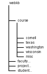
Initially, we were going to test our entire data set using random cross-validation. However, we decided that other test sets might yield interesting results. Pages from the same University might have certain traits in common. As a result, to test how our classifier might perform on pages from a University the learner had never seen, we decided to run additional experiments. Each of these additional experiments used a test set that consists of all pages from a single University and a training set that consists of all the remaining pages.

Our entire data set (4199 pages) is organized into a directory hierarchy as follows:

Figure 1 Webkb Directory Structure

Underneath Webkb/ are directories that divide the pages according to their classification. Underneath each class directory, are directories that sub-divide pages according to the Universities from which they originate. Many of the pages come from Cornell University (226 pages) and from the Universities of Texas (252 pages), Washington (255 pages), and Wisconsin (308 pages). Pages inside the misc/ directory (3158 pages) originate from Universities other than these four. We ran experiments using the following training and test sets:

Training Set	Test Set
{Webkb} - {Cornell}	{Cornell}
{Webkb} - {Texas}	{Texas}
{Webkb} - {Washington}	{Washington}
{Webkb} - {Wisconsin}	{Wisconsin}
{Webkb}	Ten-Fold Random Cross Validation

Table 1 Training and Test Sets

2.2 Feature Set Types

Typical textual classification examines occurrences of words. However, Web pages potentially contain other sources of information. For example, the number of occurrences of certain punctuation symbols might differ from the number of occurrences in regular text, and these differences might assist in classification. In addition, Web pages contain other tokens like tags that do not occur in other types of documents. In an attempt to exploit these other sources of information, we experimented with two types of feature sets:

Word counts.
Token counts.

When using word counts, each feature represented the number of occurrences of a specific word in the document. When using token counts, we allowed features to represent counts of words, punctuation symbols, html tags, and other types of tokens that a typical compiler might recognize.

2.3 Feature Selection

Once we had chosen feature types, we then needed to know exactly what words/tokens to count. We did not, for example, wish to use every unique word as a feature. We first decided to eliminate all words/tokens that did not occur at least five times in the data set, since sparse representation can skew results. We then decided to choose sets of one-thousand features according to some standard method of determining the relative usefulness of features. We discovered several techniques. Since we did not know which would perform best, we decided to try all of the following:

Average Mutual Information with respect to the class.
Point-wise mutual information with respect to the class.
Chi-Squared.

2.4 Normalization

Once we had a feature set, we needed to produce data files for input to the learner and classifier. Each data file consists of a row for each document and a column for each feature. We needed to decide what to put in the cells. Although raw counts would be useful, we thought that a certain type of normalization might give better results. For example, one might guess that a few occurrences of the word "my" would indicate a Student page or a Faculty page rather than a Course page or a Project page. However, if the document were very long, then this conclusion is less likely to be valid. We decided to try both raw counts and counts normalized for page length. The value in a given cell is either a feature count (i.e. the number of occurrences of the feature in the document) or a normalized feature count (i.e. the number of occurrences of the feature in the document divided by the total number of occurrences of words/tokens in the document). The last column in a row is the class of the document.

2.5 Summary of Parameters

We thus performed 60 experiments: (5 Data Sets) * (2 Feature Set Types) * (3 Feature Selection Mechanisms) * (2 Normalization Methods).

3 Results

This section will first consider the each parameter (e.g. Test Set, Feature Types, Feature Selection Method) separately. That is, for each parameter, we decide which value (e.g., for Feature Selection Method: average mutual information, pointwise mutual information, or chi-squared) allowed the learner to perform best. We then summarize the combinations of parameter values.

3.1 Test Set

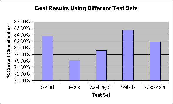
We ran twelve (60 experiments / 5 training sets) separate experiments for each test set. Figure 2 shows the best results obtained using the different test sets.

Figure 2 Best Results Using Different Test Sets

3.2 Feature Type

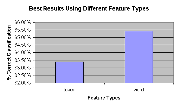
We ran thirty (60 experiments / two feature types) separate experiments for each feature set type. Figure 3 shows the best results obtained using the different feature types.

Figure 3 Best Results Using Different Feature Types

3.3 Feature Selection Method

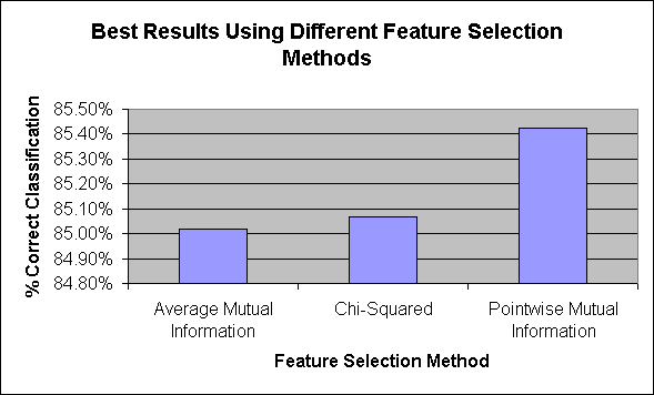
We ran twenty (60 experiments / three feature selection methods) separate experiments for each feature selection method. Figure 4 shows the best results obtained using the different feature selection methods.

Figure 4 Best Results Using Different Feature Selection Methods

3.4 Normalization

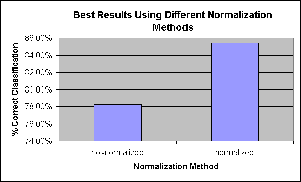
We ran thirty (60 experiments / 2 normalization methods) separate experiments for each normalization method. Figure 5 shows the best results obtained using the different normalization methods.

Figure 5 Best Results Using Different Normalization Methods

3.5 Summary of Parameters

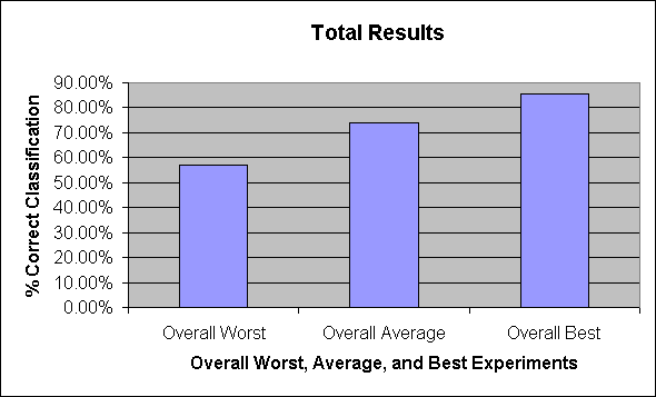
We ran a total of 60 experiments using the various values for the experiment parameters. Figure 6 shows results obtained for the worst performing experiment, the average experiment, and the best performing experiment.

Figure 6 Total Results

A complete listing of results follows:

Test Set	Feature Type	Feature Extraction	Normalized	% Correct Classification
cornell	token	Average Mutual Information	no	68.58%
cornell	token	Average Mutual Information	yes	80.53%
cornell	token	Chi-Squared	no	70.35%
cornell	token	Chi-Squared	yes	81.86%
cornell	token	Pointwise Mutual Information	no	70.35%
cornell	token	Pointwise Mutual Information	yes	81.86%
cornell	word	Average Mutual Information	no	69.91%
cornell	word	Average Mutual Information	yes	80.97%
cornell	word	Chi-Squared	no	70.80%
cornell	word	Chi-Squared	yes	81.42%
cornell	word	Pointwise Mutual Information	no	70.80%
cornell	word	Pointwise Mutual Information	yes	83.63%
texas	token	Average Mutual Information	no	57.14%
texas	token	Average Mutual Information	yes	71.83%
texas	token	Chi-Squared	no	57.54%
texas	token	Chi-Squared	yes	73.02%
texas	token	Pointwise Mutual Information	no	57.94%
texas	token	Pointwise Mutual Information	yes	71.83%
texas	word	Average Mutual Information	no	61.51%
texas	word	Average Mutual Information	yes	76.19%
texas	word	Chi-Squared	no	64.68%
texas	word	Chi-Squared	yes	76.19%
texas	word	Pointwise Mutual Information	no	57.54%
texas	word	Pointwise Mutual Information	yes	75.40%
washington	token	Average Mutual Information	no	67.45%
washington	token	Average Mutual Information	yes	73.73%
washington	token	Chi-Squared	no	69.80%
washington	token	Chi-Squared	yes	72.16%
washington	token	Pointwise Mutual Information	no	68.63%
washington	token	Pointwise Mutual Information	yes	75.69%
washington	word	Average Mutual Information	no	67.84%
washington	word	Average Mutual Information	yes	77.25%
washington	word	Chi-Squared	no	69.41%
washington	word	Chi-Squared	yes	79.22%
washington	word	Pointwise Mutual Information	no	69.02%
washington	word	Pointwise Mutual Information	yes	76.86%
webkb	token	Average Mutual Information	no	67.75%
webkb	token	Average Mutual Information	yes	82.81%
webkb	token	Chi-Squared	no	68.80%
webkb	token	Chi-Squared	yes	82.90%
webkb	token	Pointwise Mutual Information	no	68.54%
webkb	token	Pointwise Mutual Information	yes	83.40%
webkb	word	Average Mutual Information	no	69.18%
webkb	word	Average Mutual Information	yes	85.02%
webkb	word	Chi-Squared	no	69.42%
webkb	word	Chi-Squared	yes	85.07%
webkb	word	Pointwise Mutual Information	no	69.25%
webkb	word	Pointwise Mutual Information	yes	85.43%
wisconsin	token	Average Mutual Information	no	77.60%
wisconsin	token	Average Mutual Information	yes	77.27%
wisconsin	token	Chi-Squared	no	77.60%
wisconsin	token	Chi-Squared	yes	75.97%
wisconsin	token	Pointwise Mutual Information	no	76.62%
wisconsin	token	Pointwise Mutual Information	yes	79.87%
wisconsin	word	Average Mutual Information	no	77.60%
wisconsin	word	Average Mutual Information	yes	81.17%
wisconsin	word	Chi-Squared	no	76.30%
wisconsin	word	Chi-Squared	yes	81.82%
wisconsin	word	Pointwise Mutual Information	no	78.25%
wisconsin	word	Pointwise Mutual Information	yes	81.17%

Table 2 Overall Test Results

4 Conclusions

Again, we first consider each parameter separately. We then summarize which combinations of values worked best.

Test Set: The best performing experiment for each test set produced results in the 76%-85% range. Experiments using test sets corresponding to a single University performed worse than the experiment that used cross-validation. We can think of two reasons. First, the single University test sets are smaller, so a few anomalous pages can skew results. Second, as expected, it appears that the classifier has more difficulty classifying pages from a University that the learner did not see during the training process.
Feature Type: For each pair of experiments that differed only in the feature type parameter, using words consistently outperformed using words and other tokens. We surmise that using words performed better, because the tokens were so numerous that their presence began to lose meaning. For example, documents contain many more periods than occurrences of a typical word. It is somewhat disappointing that including tokens other than words did not improve performance. However, more research is needed in this area, since we did not exhaust the possibilities. For example, we counted tags. We could have been more specific and counted links, pictures, etc.
Feature Selection: Using Pointwise Mutual Information scored slightly higher than the other two methods, but scores were very close. In fact, different feature selection methods came out on top depending on other parameters for the experiments. In general, pointwise mutual information performed slightly better than the other two feature selection methods.
Normalization: Using normalized counts consistently performed significantly better than using un-normalized data. This result is reasonable. Again, one would expect a page with a few occurrences of the word "my" to indicate a student page or a faculty page, but not necessarily if the page were 50,000 words long.

Best results made use of the following combination of parameter values:

Test Set: Webkb Ten-Fold Stratified Cross Validation

Feature Types: words only

Feature Selection Method: pointwise mutual information

Normalization: normalized for page length

The best performing experiment achieved approximately 85% correct classification. These results were better than the 40% results obtained by Carnegie Mellon researchers [Craven et. all]. However, the CMU researchers attempted to classify pages into seven categories, while we used only four categories.

Again, Naive Bayes proves itself a good way to classify textual documents. 85% classification is a good start at attempting to learn from the Web.

5 Related Work/Literature

[1] Webkb Data Set

[2] JLex

[3] Weka Tools

[Craven et. all] M. Craven, D. DiPasquo, D. Freitag, A. McCallum, T. Mitchell, K. Nigam, S. Slattery. 1998. Learning to Extract Symbolic Knowledge from the World Wide Web.

Mitchell, Machine Learning, WCB/McGraw-Hill, 1997.

Witten, Frank, Data Mining, Morgan Kaufmann, 1999.

Send comments to: Mark Chavira and Ulises Robles-Mellin
Last modified: Mon. Mar 13, 2000