In order to compare the performance
of different metric constraints to a real reference, synthetic data was
used in the first part of the experiment. The camera motion goes
around the randomly generated 80 object points in half an elliptical path.
The size of the 80 points range from -2 to -2 in their x and y coordinates.
The lengths of the main axis of the ellipse are 16 and 12. A Gaussian
noise source having variance of 0.5 was added to the data in the image
frame. A total of 162 frames were generated from this configuration.
Figure (1) shows the recovered camera
rotation. Note that the motion recovery from the three methods are
all very close to the real camera motion (in blue). In most cases,
the recovered motion from the scaled orthography matches almost exactly
with the paraperspective assumption. However, both methods start
to deteriorate when the scale of the object is small compared to the camera
distance. This was not expected since this is one of the assumptions
from which these methods are derived. Further investigation is needed
in this area.
 |
|
red- scaled orthography, yellow - paraperspective. Top: yaw, middle: pitch, bottom: roll. |
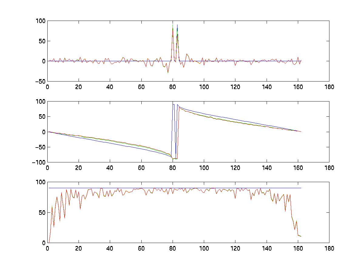
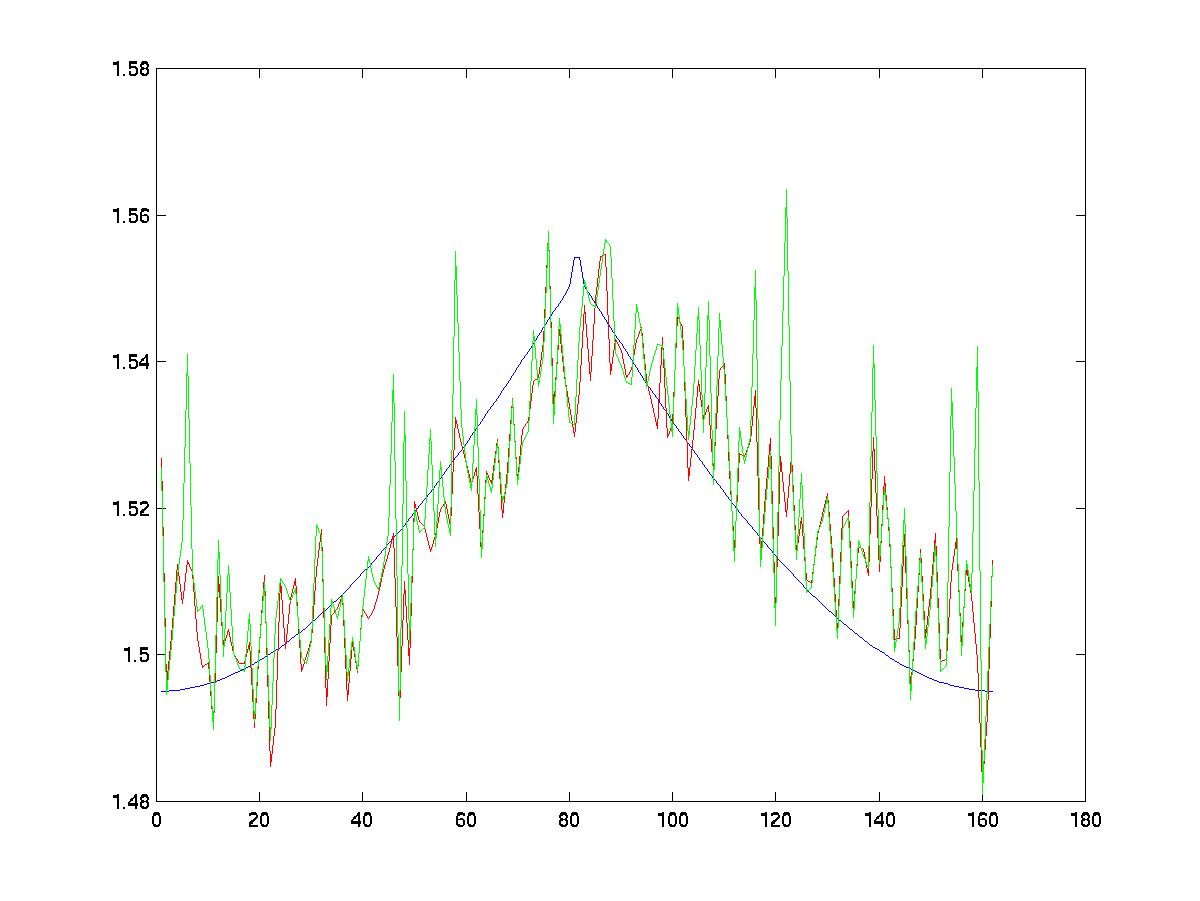
Figure (2) shows the estimated camera
depth using perspective approximation. The blue line is the real
camera depth, scaled arbitrarily to match the shape of the estimated camera
depth. Note that the scaled orthography works better in this particular
case. The paraperspective approximation measurement is very noisy;
consequently, the estimated camera depth has spikes in almost any place.
 |
|
|
The recovered object shapes from these
factorization are hard to visualize because the points are randomly generated.
Furthermore, the recovered shapes are only correct up to a scale factor,
making it more difficult to be compared. We will look at recovered
object shape from the real data in the following section.
We tested the factorization method
on a real image sequence taken from the CMU
VASC image database. The hotel sequence consists of a set of
frames of a small model building moving around in front of the camera.
We first used a KLT tracker (code written in C, provided by Professor Tomasi)
to track the features. In the hotel image sequence, 250 features were tracked,
while 210 of them were used for the motion/shape recovery.
All three methods were applied to the hotel sequence. The results are shown in figure (3) - (5). Unfortunately, the paraperspective project method failed for this particular image sequence. The G = Q*Qt matrix in equation (3) (see the Factorization method section) turned out to be non-positive definite and thus we could not simply calculate the Jacobi Transformation and take the square root. One can solve the problem by means of an iterative method called Newton's method [4]. For time constrained reasons, we did not explore this option in the project. Moreover, we also encountered that the image sequence does not contain enough translation along the optical axis or it contains too much measurement noise.
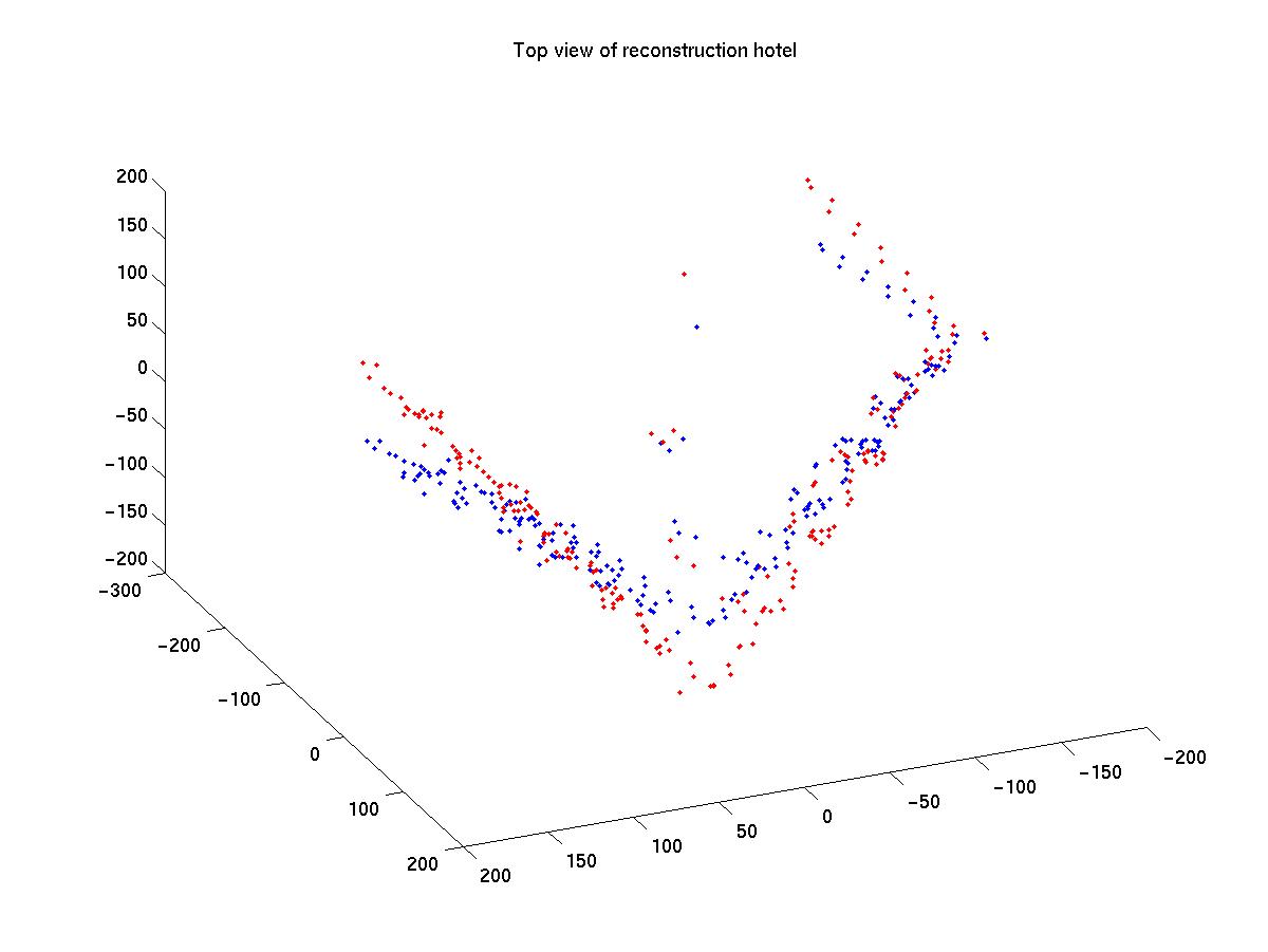
Figure (3) shows the bottom view
of the reconstructed hotel. It is easy to see that the scaled orthographic
assumption (shown as red in the graph) performs better in that each wall
is more perpendicular to its neighbor. This is expected because the
scaled orthographic assumption takes into account that there is small camera
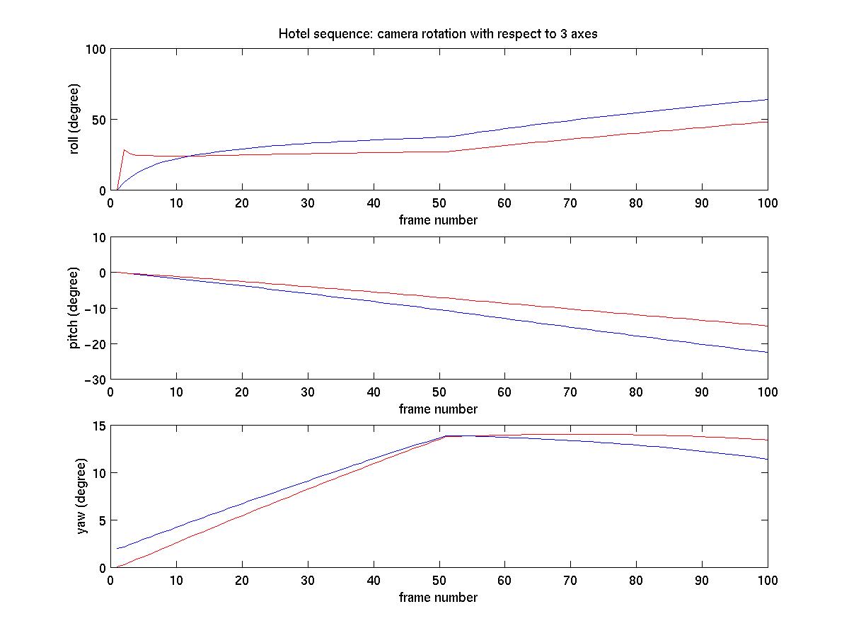
motion along the direction of optical axis. Figure (2) shows the
estimated camera rotation about the three axes. Note there is change
in motion around frame 50. This change can be observed in the hotel
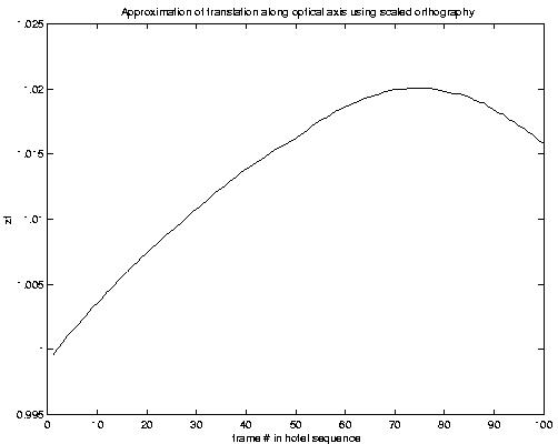
image sequence (11M QuickTime movie). Figure(3) shows the estimated
translation in the z direction using the scaled orthographic projection
method. The camera seems to be getting slightly closer to the object as
time goes on. This estimate is not available in the orthographic
assumption.
 |
|
blue - orthographic projection., red - scaled orthographic projection |
 |
|
Again, blue - orthographic proj., red - scaled orthographic projection. |
 |
|
|
We had to modify the code that implements the Factorization method. The first problem was that the sequences were mostly non-normalized for the factorization method. We solved this by adding 1 to the diagonal elements of the matrix Q before computing its square root (see Factorization Method section). Another problem was the singularity of some matrices, which we solved by floor-ing (i.e, rounding down) the elements in the matrices. This reduced a bit the quality of the results.
We did not use any heuristic in order to find the "best" submatrix W for a given missing point (see Occlusion section). We used exhaustive search to find the first three points that satisfy the reconstruction constrain and we stopped the search once we found them.
We run the code for occlusion varying the
number of features (60,100 and 250) and the results are as presented as
follows:
|
|
Number of Frames | Total Points | Number of Original Missing Points | Number of Missing points after running "occlusion" | % Of Total points that are known after running "occlusion" |
|
|
160 | 40,000 | 27,618 | 636 | 98.41 |
| 250 | 100 | 25,000 | 13,904 | 396 | 98.41 |
| 250 | 60 | 15,000 | 6,427 | 236 | 98.42 |
| 100 | 160 | 16,000 | 12,115 | 1,722 | 89.23 |
| 100 | 100 | 10,000 | 6,345 | 297 | 97.03 |
| 100 | 60 | 6,000 | 2,986 | 177 | 97.05 |
| 60 | 160 | 9,600 | 7,634 | 1,513 | 84.23 |
| 60 | 100 | 6,000 | 4,103 | 982 | 83.63 |
| 60 | 60 | 3,600 | 1,929 | 128 | 96.44 |
Table 1. Results on the performance of the implementation of occlusion over some number of frames and points.
In Table (1) we see that the data
set has a lot of unknowns. The algorithm performs better when we have more
frames and points; although sometimes its performance is not very good.
We think that in these cases there are not enough points that can be found
to satisfy the reconstruction condition, but if the number of frames increases,
we can recover more data, since more points will satisfy the condition.
We also noticed that the results reach convergence as the number of frames
to consider grows.
 |
|
|
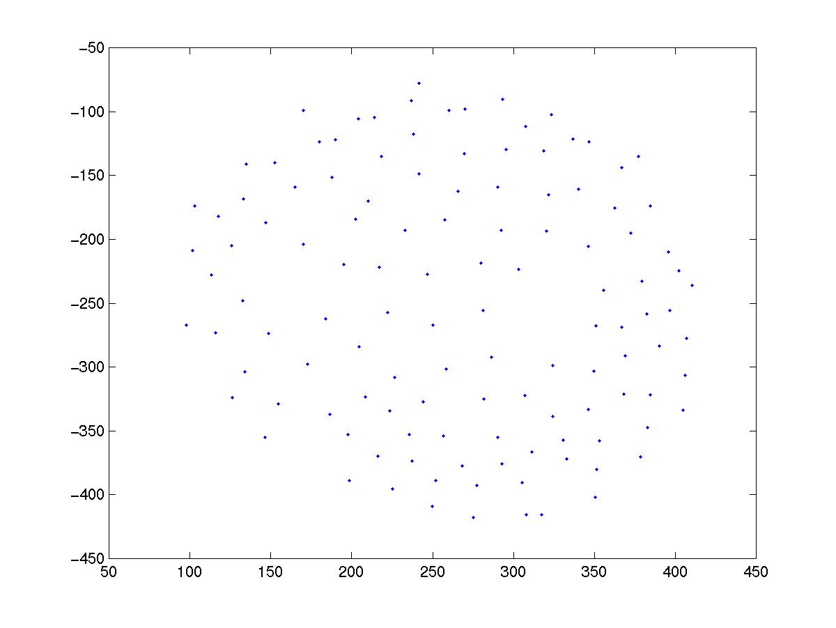
Figure (6) shows one screen-shot gotten when running the algorithm for 250 points and 160 frames. In order to display the results and make the simulation, we divided the data in 2 halves (125 points each in this case). Of those 125 points in the matrix, we could recover 121 of them as this screen-shot shows.
The drawbacks of this implementation are
that we could not run the code for tracking more than 160 frames,
so we could not see the performance in considering further frames, but
the tendency demonstrates that using more computational power, we could
nearly reconstruct all points if the number of frames is big enough.
Another issue is that we sometimes had to round up the matrices S and R
(from the Factorization algorithm) in order to get the code working
and to avoid singular matrices. This might also affect the results. Finally,
we used exhaustive search as mentioned above. If we had used any heuristic,
we should have found the missing points faster.
![]()
![]()
![]()
Next: SummaryPrevious: Occlusion Contents: Shape and Motion from Image Streams