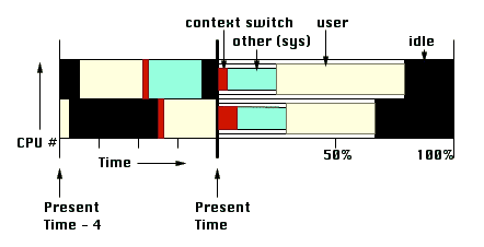
Figure 1: Current Trends (CT) and Summary of History (SH) plots for processor usage
This paper is based on the idea that the operating system and processes in the system can be visualized through resource usage. We discuss design issues in the context of process visualization and look at some existing systems for this purpose. The main focus is the development of a new visualization incorporating the principles we have established through discussion of the design issues and existing systems.
A process is a program in execution, needing resources to perform its task. These resources include the CPU, memory, storage (such as disk space), I/O devices and ports for communication. Visualizations of system resource usage will therefore help in understanding program execution and in identifying possible problems and ways to correct them. Since resources are typically allocated by the operating system, such visualizations are also a useful tool for analysis of system performance.
This paper discusses general design techniques which might be useful for visualizing processes and systems, looks at some existing visualizations of resource usage and proposes new visual metaphors in this context. It is important to remember that the focus here is on visual metaphors, not on data collection, though the latter is a very important aspect of any system simulation.
The paper is structured around the design of a new visualization. Issues are examined as they arise in this design - the decisions taken by existing systems on these issues are discussed, and accepted / rejected in the new system on the basis of this discussion.
A process is different from a program in that it is an active entity. Besides the program code that it executes, it consists of its context -
These relate in a simple way to system resources. The process state, PC, CPU registers and scheduling information describe CPU usage, the data section and memory management information refer to memory usage and I/O status information relates to I/O device usage. This is the rationale for using resource usage to visualize processes.
The other part of a process is the passive component - the program code. We will not discuss this aspect of the process. Tools such as Seesoft [ESS92], when integrated with resource views, will provide a complete process visualization.
The visualization of processes and the system described in this paper are intended to be used in the context of a system simulation package such as SimOS or Performance Co-Pilot. The data required is assumed to be stored in a log file, and the speed/detail trade-off feature of SimOS is assumed to be present.
If data acquisition is being done in real time, the obvious change required is a limit on the detail of the visualization. Since the speed of the visualization is variable (see Section 2.4), we will also need a limit on the lag of the visualization relative to actual system time. This means that the user has a choice of losing information from a time period in the future (if he/she freezes the visualization or runs it at too slow a speed) or from the present (if he/she catches up with the system).
In this section, we discuss design issues that arise in process visualization, some design choices made by existing visualizations and why these choices are appropriate or inappropriate in the context of process and system visualization.
Screen space is extremely limited, especially when considered relative to the enormous amounts of data that need to fit into it in resource usage visualization. One way of managing screen space is to use a windowing system, as in PROVIDE [Moh88] and Program Visualizer [KRR94] where a separate window is used for each graph or piece of information. There are significant problems with this method. When there are a large number of entities, some will be obscured by others and will be difficult to find. There are graphs which are much more useful when placed in certain positions relative to others - this placing will have to be done manually.
An alternative, and better, method is to form groups of graphs (allow sharing) and display them separately, similar to the Rooms interface [CH87]. Though the Rooms interface was designed for user task switching, it is useful in fairly general situations to avoid the clutter of a pure windowing system. In our visualization, the automatically-generated rooms contain standard graphs pertaining to one or more system resources. This set of rooms can be kept fully connected (i.e., there are doors from every room to every other room) since there are not many of them.
Any visualization design should use the design principles laid down in [Tuf91] and [RT96]. Two specific issues which arise in the context of system and process visualization are mentioned below.
A lot of the situations involve partitioning data into classes - an example is the partitioning of memory into regions used by different processes. In a more general visualization system, metadata would need to be used to decide how many classes would be appropriate. In our more restricted situation, however, we already know certain things about our data. Since memory can be considerably fragmented, we are better off dividing memory into regions which are being used by the kernel, those which are being used by any user process and those which are currently unused, instead of using a finer division.
Focusing on a process (or a group of processes) in our design is equivalent to highlighting the data associated with the process (or the group). This highlighting should be done with a color which is sufficiently different in hue from the other processes, to provide a visual cue for qualitative difference. When showing quantitative data using color such as in a colored matrix, the magnitude is represented by luminance - the use of an isomorphic colormap is essential for correct interpretation.
We always try and place graphs with common axes stacked against each other so that variations in the other variables can be compared and correlated. For instance, time is a variable in a large number of the graphs we use - whenever possible, we stack these graphs vertically.
A VCR paradigm is fairly appropriate to represent time and its passage in almost any visualization - especially one in which most plots have a common time axis. We allow the user to smoothly vary the speed of the visualization, including a total freeze at any time instant. This is similar to the control panel in the Program Visualizer.
Further, we represent all time axes as relative to the present time - this implies sliding axes, with plots showing data collected from a fixed time before the present (user-adjustable) to the present time. This kind of sliding axis is common in case of CPU usage; we, however, also use it in other situations such as memory maps (see Section 3.3).
It takes extra effort and time on the part of the user to understand 3-dimensional plots (using animation to change the angle of view, say). Besides, they take up more display space, thus giving a lower information density. Another disadvantage is that they cannot be placed beside each other and compared without first matching angles of view, which may obscure some quantities while highlighting others.
We have therefore eliminated these plots from our design, choosing to represent the third dimension in a form other than spatial. In situations which require a comparison in two dimensions, the Performance Co-Pilot system uses 3-dimensional bar charts along with a color component segmenting the magnitudes represented by the heights of the bars. There is redundancy involved in this representation - we use 2-dimensional colored matrices instead in our visualization. This is a simpler design which is, at the same time, easier to understand.
A specific user's needs could be very different from the designer's idea in any system design. In the case of resource usage visualization, the graphs described in the following sections might not serve the user's purpose well. We therefore need to make the visualization flexible. In our design, this can be accomplished by providing mechanisms to define new quantities, new graphs, and new rooms. New quantities can be defined by allowing application of arithmetic and aggregate operators on existing quantities, new graphs by plugging metrics (newly created or originally present) in graph templates, and new rooms by selecting sets of graphs (newly created or originally present).
The simplest visualization results when there is no process "in focus". This view is useful for analyzing system performance - it consists of a process tree and a component for each resource. We would like the resource-dependent components to provide us with summaries of the history of their usage so far. Another desirable is the current trends in their usage. We therefore develop a summary of history (or SH) graph and a current trends (or CT) graph for each of the resources we visualize in this section (processors, memory, and I/O devices).
An overview of the system needs to show the processes in the system. This hierarchy is not used in analyzing performance, but it allows future selection of processes to focus on. The Program Visualizer has a process tree window which displays the process hierarchy in the conventional way. As is clear from the screen snapshot, this occupies too much display space. A much better option is the hyperbolic view presented in [LRP95] which lays out the hierarchy on a hyperbolic plane and maps the plane onto a disk.
In the case of CPU usage, the current trends plot is a conventional band graphs of CPUs versus relative time (as in SimOS), color coded by the state of the CPU:
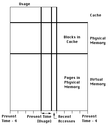
Memory is usually shown as an array of pages / blocks, color coded according to usage. Some systems try to show as many distinctions in memory usage as possible often leading to clutter. We divide memory usage into just three classes - that used by the operating system, that used by any user process and that which is unused. We do however mark boundaries between regions allocated to different processes - this reveals information about memory fragmentation without increasing clutter.
This conventional view neither shows the past history of the memory nor what
the current trends are, though they may be understood by carefully observing
change in the array with time. To make the user's task easier, we use a
sliding time axis showing usage at recent times. We also use a
The summary of the history consists of miss rates for each level of the memory hierarchy.
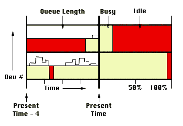
To reduce clutter and to cull non-essential information, the user should be able to select subsets of I/O devices. The graphs for this chosen subset of I/O devices are similar to those for CPU usage, with idle / busy being the only distinction of state. The CT plot includes an extra quantity - the length of the queue for the device.
Analysis is considerably eased if all the information is present together, but there is never enough screen real-estate to allow this without clutter. The memory display probably needs to be by itself; the CPU and I/O device usage can be shown together or separately.
The process tree of Section 3.1 can be used to select a set of processes to focus on. Focusing causes all current trend plots in the system overview to make a further distinction - that between selected and unselected processes.
Summaries of history are more difficult to handle because they depend on all the data in the log file upto the current point. The user can optionally change SH graphs to consider only the selected processes for percentages / averages. However, these percentages / averages can only be computed from the point of selection of this option - doing otherwise would require re-reading the entire log file.
Besides these changes, there will now be an additional process comparison (PC) graph for each resource. We also discuss some other graphs which would be useful in understanding process performance.
The process comparison plot for processor usage is a color coded matrix with processors on one axis and (selected) processes on the other. The color (we use an isomorphic luminance colormap) indicates the percentage of its running time a process has spent on a processor. The matrix permits comparison of time spent by a process on different processors, and of the loads of different processors.
The visualization also includes another new color coded matrix - that of (selected) process against process state (running, ready, waiting). The color in the matrix gives the percentage of time spent by a process in a state. An extra row giving process priorities helps in interpreting the matrix.
| Priority | . | . | . | ||
|---|---|---|---|---|---|
| Process State | . | . | . | ||
| . | . | . | |||
| . | . | . | |||
| CPU # | . | . | . | . | . |
| . | . | . | . | . | |
| . | . | . | . | . | |
| Process # | -------- Time -------- | ----- Percentage ----- | |||
The process comparison graph is similar to that for processor usage - it is a matrix of process against miss rate for each level of the hierarchy.
| Level # | . | . | . | . |
|---|---|---|---|---|
| . | . | . | . | |
| Process # | --- Miss Rate (%) --- | |||
There are two PC matrices for I/O devices. They show respectively the number of requests made and the time spent waiting in the queue for each (selected) I/O device for each (selected) process.
| # of requests | waiting time | |||||||
| Device # | . | . | . | . | . | . | . | . |
|---|---|---|---|---|---|---|---|---|
| . | . | . | . | . | . | . | . | |
| . | . | . | . | . | . | . | . | |
| Process # | Process # | -------- Time -------- | ----- Percentage ----- | |||||
This visualization helps when the selected set of processes is a co-operating group. In a message-passing system, the PC graph is a simple matrix of selected process against selected process, the color giving the number of messages passed.
Current trends are visualized with another process - process matrix where any communication is represented by a high-luminance color which fades with time. This technique is the same as that used in Section 3.3 to show memory accesses.
| # of messages | recent messages | |||||
| Process # | . | . | . | . | . | . |
|---|---|---|---|---|---|---|
| . | . | . | . | . | . | |
| . | . | . | . | . | . | |
| Process # | Process # | |||||
Even if we display all the different resources discussed in this section in different rooms, there is no problem with navigation. However, the user may want to create additional rooms with different groupings or with wholly new plots. In this situation, we ask the user to specify the doors from and to the new rooms.
We have taken the view that the operating system is a resource provider and the process is a resource user. With this very simple picture which is not very far removed from the real situation, resource usage is an appropriate concept for analysis of both operating system and process performance.
We have looked at common design issues in system visualizations and discussed existing and new visual metaphors. The flexibility issue has been very cursorily examined. Important issues which have NOT been discussed include data collection and program code visualization. A design has been developed by assuming a data collection system and excluding program code visualization.
Design processes are typically iterative - the design developed in this paper is a first iteration and will benefit from feedback and further thought.