Grids are commonly used in games for representing playing areas such as maps (in games like Civilization and Warcraft), playing surfaces (in games like pool, table tennis, and poker), playing fields (in games like baseball and football), boards (in games like Chess, Monopoly, and Connect Four), and abstract spaces (in games like Tetris). I’ve attempted to collect my thoughts on grids here on these pages. I avoid implementation details (such as source code) and instead focus on concepts and algorithms. I’ve mostly used grids to represent maps in strategy and simulation games. Although many of the concepts here are useful for all sorts of grids, there is a bias towards the kinds of games I am interested in.
Grids are built from a repetition of simple shapes. I’ll cover squares, hexagons, and triangles[2]; vertices, edges, and faces (tiles); coordinate systems; and algorithms for working with grids. The impatient should skip ahead to coordinate systems. I also have a guide to hexagonal grids[3] with many more hex-specific algorithms.
Squares
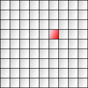
The most common grid is a square grid. It’s simple, easy to work with, and maps nicely onto a computer screen. Square grids are the most common grids used in games, primarily because they are easy to use. Locations can use the familiar cartesian coordinates (x, y) and the axes are orthogonal. The square coordinate system is the same even if your map squares are angled on screen in an isometric or axonometric projection.
Hexagons
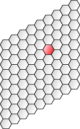
Hexagons have been used in some board and computer games because they offer less distortion of distances than square grids. This is in part because each hexagon has more non-diagonal neighbors than a square. (Diagonals distort grid distances.) Hexagonals have a pleasing appearance and occur in nature (for example, honeycombs). In this article, I’ll use hexagons that have flat tops and pointy sides, but the math works the same if you want pointy tops and flat sides. I also have a more comprehensive guide[4] that covers offset coordinates, axial coordinates, cube coordinates, pointy tops, flat tops, and many more algorithms.
Triangles
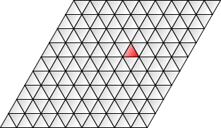
Triangles are common in 3D graphics but are rarely used for game maps. A big disadvantage of triangle maps, aside from unfamiliarity, is the large perimeter and small area (the opposite of a hexagon). The small area means it’s harder to place game pieces completely within a single space on the map. In 3D graphics, triangles are the only shape that is planar; squares and hexagons can be “bent”, sometimes in impossible ways. In this article I’ll use triangles pointed up and down, but the math works the same if your triangles point left and right.
Grid Parts#
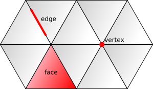
Grids have three types of parts: faces (tiles), edges, and vertices. Each face is a two dimensional surface enclosed by edges. Each edge is a one dimensional line segment ending at two vertices. Each vertex is a zero dimensional point. It is common for games to focus on only one of these types of parts. “Western” games like Chess and Checkers seem to focus on faces and “eastern” games like Go and Chinese Checkers seem to focus on vertices. There are some games like Roulette that assign meaning to all three types of grid parts.
Faces, edges, and vertices show up in polygonal maps as well. Algorithms that work on faces, edges, and vertices without requiring grid coordinates will work on these polygonal maps:
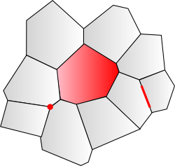
Grids and polygonal maps can be converted into graph structures by turning each face into a node and each edge between faces into a graph edge between nodes. The graph structure allows the use of graph algorithms (such as shortest path) on the grid map.
Uses in games
Computer games can use all three types of grid parts, but faces are the most common. Buildings, land types (grass, desert, gravel, etc.), and territory ownership use faces. Territory borders and “flow” algorithms (which simulate the flow of water, people, goods, etc., between adjacent faces) can use edges. Heights (altitude, water depth) use vertices. Roads and railroads can either use faces (as in SimCity) or edges (as in Locomotion; see my Java applet demonstrating this[5]).
Counting the parts
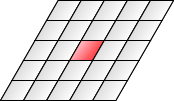
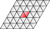
We can count how many faces, edges, and vertices are needed to form a grid. The approach is to look at adjacency and sharing. Consider a triangle grid (see Figure 4). Each triangle face has 3 edges. Thus, we expect 3 times as many edges as faces. However, each edge is shared by 2 faces, so we have 3 edges for every 2 faces. Each triangle face has 3 vertices (corners). Each vertex is shared by 6 faces. Therefore we have 3 vertices for every 6 faces, or 1 vertex for every 2 faces. These relationships will be important when designing coordinate systems. Squares have equal numbers of faces and vertices. Hexagons have more vertices than faces. Triangles have more faces than vertices. There are always more edges than faces or vertices.
| Shape | Faces (F) | Edges (E) | Vertices (V) |
|---|---|---|---|
| square | 1 | 2 | 1 |
| hexagon | 1 | 3 | 2 |
| triangle | 2 | 3 | 1 |
I’ll call these the F,E,V counts. The F,E,V of squares is 1,2,1; of hexagons, 1,3,2; of triangles 2,3,1. Notice that hexagon and triangle grids have similar counts, except the vertices and faces counts are reversed. That’s because hexagon grids and triangle grids are duals: if you place a vertex in the center of each face of a triangle grid, you will get a hexagon grid, and vice versa. Square grids are duals of themselves. If you place a vertex in the center of each square, you will produce another square grid, offset from the first. Read more about duals on Wikipedia[6].
Derivation of Hexagon and Triangle Grids#
Hexagon and triangle grids can be derived from square grids. (Try changing the angle in this Flash demo[7].) Since coordinate systems for squares are straightforward, the derivation will guide us in designing coordinate systems for hexagons and triangles.
Squares to Hexagons
There are two steps needed to turn a square grid into a hexagon grid. First, we must offset the columns (or rows). Second, we split half the square edges and bend them in the middle.
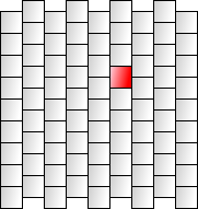
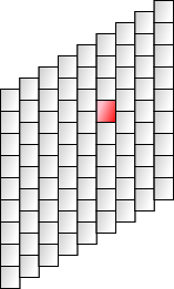
There are two simple ways to offset columns. The most common is to offset every other column (see the first grid in Figure 5). Code using this approach looks at whether it’s an odd or even column and chooses whether to offset it. A simpler approach is to offset each column by half a height more than the previous column (see the second grid in Figure 5). Code using this approach is more uniform, but the map shape is no longer rectangular, which can be inconvenient. On these pages I will focus on the latter approach; it’s easier to work with and can be also used with triangles. (In a future version of this page I may cover the other form as well.)

With either offset approach, the next step is to split the vertical edges of the squares and bend them, as shown in Figure 6. When the bend is reduced from 180 degrees to 120 degrees, you will have regular hexagons. Note that splitting the vertical edges means we’ve increased the number of edges from 4 to 6 (a net increase of 1 edge per face, since the 2 new edges are shared by 2 faces). We’ve also increased the number of vertices from 4 to 6 (but these vertices are shared, so the net increase is 1), and we’ve left the number of faces unchanged. The F,E,V counts go from 1,2,1 to 1,3,2.
Squares to Triangles
There are two steps needed to turn a square grid into a triangle grid. First, we must shear[8] the squares. This gives us a rhombus grid (see Figure 7). To make triangles we split each rhombus face into two triangles. Splitting each face means we now have twice as many faces as before, we’ve added 1 edge for each face, and we haven’t added any vertices. The F,E,V counts go from 1,2,1 to 2,3,1.
Coordinate Systems#
There are three grid parts, and we need a way to address each of them. I’ll start with simple numeric coordinates that match the grid’s axes. The F,E,V counts tells us how many grid parts share the same coordinate. If more than one part has the same coordinate, I’ll use a capital letter to disambiguate.
Square Grids
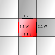
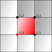
Square grids are fairly easy. See the first diagram in Figure 8
for the standard coordinate system for faces. The F,E,V counts
are 1,2,1. That means only edges will need a letter for
disambiguation. For every face we (arbitrarily) assign one
vertex to share its coordinate. I’ve chosen the southwest
corner of the face. Compare the face diagram to the vertex
diagram to see how the coordinates are related. For each face
we assign two edges to share its coordinate. I’ve chosen the
south and west edges, and annotated the coordinates with the
letters S and W. Compare the face
diagram with the edge diagram to see how the coordinates are
related. There is one face, two edges, and one vertex that
share the (1, 1) grid coordinate. This matches our F,E,V counts
of 1,2,1.
Hexagon Grids
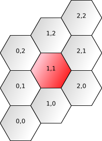
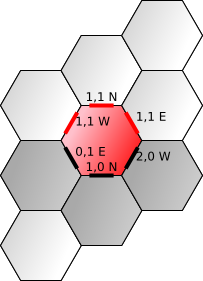
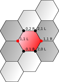
We created the hexagon grid out of a square grid. The coordinates of a hexagon face can be the same as the coordinates of the square face that was transformed into that hexagon. Compares Figure 8 to Figure 9 and you can see how the face coordinates are related. For each face we choose three edges and two vertices to share the same coordinate. I’ve chosen the NW, N, and NE edges, and labeled them W, N, E. I’ve chosen the leftmost and rightmost vertices and labeled them L, R. Many other assignments are possible.
Triangle Grids
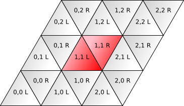
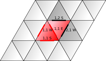
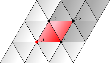
We created a triangle grid out of a square grid, and we split each sheared square (rhombus) into two triangles. This means each square face coordinate needs to be two triangle face coordinates. I chose to label them L and R, as seen in Figure 10. The edges are the same as those for squares (W and S), except we have one additional edge from the splitting of the face in two, and I’ve labeled that E. The extra triangle face does not create any additional vertices, so the vertex labeling is the same as the square grid labeling.
There’s another scheme described here[9] that I need to study. It seems simpler than what I have here. And also see this scheme[10] - elegant approach when your map is a triangle.
Relationships between Grid Parts#
Given each of the 3 grid parts, we can define relationships with 3 grid parts, giving us 9 relationships. There are more relationships you can define, but I’ll focus on these 9. I don’t know the standard names for these relationships, so I’ve made up some names.
| Part A (black) | Part B (red) | ||
|---|---|---|---|
| Face | Edge | Vertex | |
| Face | Neighbors: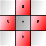
|
Borders: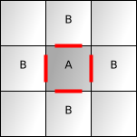
|
Corners: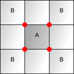
|
| Edge | Joins: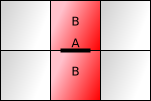
|
Continues: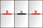
|
Endpoints: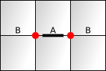
|
| Vertex | Touches: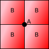
|
Protrudes: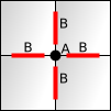
|
Adjacent: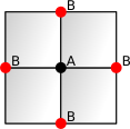
|
In your game you may want to use variants of the above. For example, the neighbors and adjacent relationships could have included diagonals. The continues relationship could have included edges that weren’t colinear with the original edge. I chose the simplest relationships.
A reader suggests connects instead of continues as a name that works better for hexagonal grids.
Algorithms
Each of these 9 relationships can be expressed in as algorithms from A to a list of Bs; I write them as A → B1 B2 B3… . There are 3 shapes, so that gives us 27 potential algorithms, expressed here in a simple form that you can translate into your favorite programming language. For some shapes and algorithms, there is more than one variant of A, so I will list the rules for each variant. For example, triangle faces come in L and R variants. Here are all the algorithms:
| Relationship | Shape | ||
|---|---|---|---|
| Square | Hexagon | Triangle | |
| Neighbors:
|
(u,v) → (u,v+1) (u+1,v) (u,v-1), (u-1,v) | (u,v) → (u,v+1) (u+1,v) (u+1,v-1) (u,v-1) (u-1,v) (u-1,v+1) | (u,v,L) → (u,v,R) (u,v-1,R) (u-1,v,R) (u,v,R) → (u,v+1,L) (u+1,v,L) (u,v,L) |
| Borders:
|
(u,v) → (u,v+1,S) (u+1,v,W) (u,v,S) (u,v,W) | (u,v) → (u,v,N) (u,v,E) (u+1,v-1,W) (u,v-1,N) (u-1,v,E) (u,v,W) | (u,v,L) → (u,v,E) (u,v,S) (u,v,W) (u,v,R) → (u,v+1,S) (u+1,v,W) (u,v,E) |
| Corners:
|
(u,v) → (u+1,v+1) (u+1,v) (u,v) (u,v+1) | (u,v) → (u+1,v,L) (u,v,R) (u+1,v-1,L) (u-1,v,R) (u,v,L) (u-1,v+1,R) | (u,v,L) → (u,v+1) (u+1,v) (u,v) (u,v,R) → (u+1,v+1) (u+1,v) (u,v+1) |
| Joins:
|
(u,v,W) → (u,v) (u-1,v) (u,v,S) → (u,v) (u,v-1) |
(u,v,N) → (u,v+1) (u,v) (u,v,E) → (u+1,v) (u,v) (u,v,W) → (u,v) (u-1,v+1) |
(u,v,S) → (u,v,L) (u,v-1,R) (u,v,E) → (u,v,R) (u,v,L) (u,v,W) → (u,v,L) (u-1,v,R) |
| Continues:
|
(u,v,W) → (u,v+1,W) (u,v-1,W) (u,v,S) → (u+1,v,S) (u-1,v,S) |
No edges continue straight in a hexagonal grid | (u,v,W) → (u,v+1,W) (u,v-1,W) (u,v,E) → (u+1,v-1,E) (u-1,v+1,E) (u,v,S) → (u+1,v,S) (u-1,v,S) |
| Endpoints:
|
(u,v,W) → (u,v+1) (u,v) (u,v,S) → (u+1,v) (u,v) |
(u,v,N) → (u+1,v,L) (u-1,v+1,R) (u,v,E) → (u,v,R) (u+1,v,L) (u,v,W) → (u-1,v+1,R) (u,v,L) |
(u,v,W) → (u,v+1) (u,v) (u,v,E) → (u+1,v) (u,v+1) (u,v,S) → (u+1,v) (u,v) |
| Touches:
|
(u,v) → (u,v) (u,v-1) (u-1,v-1) (u-1,v) | (u,v,L) → (u,v) (u-1,v) (u-1,v+1) (u,v,R) → (u+1,v) (u+1,v-1) (u,v) |
(u,v) → (u-1,v,R) (u,v,L) (u,v-1,R) (u,v-1,L) (u-1,v-1,R) (u-1,v,L) |
| Protrudes:
|
(u,v) → (u,v,W) (u,v,S) (u,v-1,W) (u-1,v,S) | (u,v,L) → (u,v,W) (u-1,v,E) (u-1,v,N) (u,v,R) → (u+1,v-1,N) (u+1,v-1,W) (u,v,E) |
(u,v) → (u,v,W) (u,v,S) (u,v-1,E) (u,v-1,W) (u-1,v,S) (u-1,v,E) |
| Adjacent:
|
(u,v) → (u,v+1) (u+1,v) (u,v-1) (u-1,v) | (u,v,L) → (u-1,v+1,R) (u-1,v,R) (u-2,v+1,R) (u,v,R) → (u+2,v-1,L) (u+1,v-1,L) (u+1,v,L) |
(u,v) → (u,v+1) (u+1,v) (u+1,v-1) (u,v-1) (u-1,v) (u-1,v+1) |
Relations
(Feel free to skip this section.) The relationships listed above are themselves related to each other. For example, borders goes from faces to edges, and it’s the inverse of joins, which goes from edges to faces. If some edge B is in the borders list of some face A, then A will be in the joins list of edge B. These 9 relationships can be distilled down into 6 mathematical relations.
If you had a database, you could express the relations directly. For example, here’s the relation between faces and edges in a small 1x2 square grid:
| Face | Edge |
|---|---|
| 0,0 | 0,0,S |
| 0,0 | 0,0,W |
| 0,0 | 0,1,S |
| 0,0 | 1,0,W |
| 1,0 | 1,0,S |
| 1,0 | 1,0,W |
| 1,0 | 1,1,S |
| 1,0 | 2,0,W |
Given a relation, you can look things up in any column. For
example, with the above table, looking up
Face==(0,0) results in 4 edges, which is what the
borders relationship expresses. Looking up
Edge==(1,0,W) results in 2 faces, which is what the
joins relationship expresses. A relation is
more general, and allows you to look things up in many ways;
each relationship (and algorithm) is an expression of one
particular way of looking things up.
Given 6 relations, there should then be 12 relationships. Why do we have only 9? It’s because the Face/Face, Edge/Edge, and Vertex/Vertex relations are symmetric, so looking things up the other way produces the same answer. Thus, 3 of the 12 relationships are redundant, and we are left with 9.
Implementation
All the algorithms are straightforward. How might you implement
them? You’ll first want to choose data structures for each of
the three coordinate systems. I recommend keeping it very
simple and transparent. All the coordinate systems I listed
have an integer u and an integer v,
and some of them have an annotation like L or
W. For the structure, in Ruby use a class with
public attrs; in Lisp use a list; in C use a struct; in Java use
a class with public fields; in Python use a simple object or
dict. For the annotations, in Ruby or Lisp, use symbols
('L or :L); in C, use characters
('L') or an enum type (L); in Java,
use characters; in Python, use one-character strings.
The next step is to implement the algorithms you need. The simplest thing to do is to write functions (or methods) that take A and return a list of B. If there are multiple variants of A, use a switch/case statement to branch on the annotation. This is the simplest approach, but it is not the fastest. To make things faster, your caller might pre-allocate the list, or you might provide a callback that is inlined (for example, STL function objects in C++). In some situations you’ll want to look up many As at once, so you might provide an algorithm that works on lists of A and produces lists of lists of B.
I generally avoid giving implementations, because they are too
specific to each game, but I’ll give an example of the Triangle
shape in Ruby. I chose to use a list as my basic data
structure, and I use Ruby symbols (like :L) for
annotations.
| Algorithm | Ruby Code |
|---|---|
|
(u,v,L) → (u,v+1) (u+1,v) (u,v) (u,v,R) → (u+1,v+1) (u+1,v) (u,v+1) |
  def corners(face)
    u, v, side = face
    case side
    when :L
      [[u, v+1], [u+1, v], [u, v]]
    when :R
      [[u+1, v+1], [u+1, v], [u, v+1]]
    end
  end
|
It’s that simple. Each variant becomes a case in the
case statement.
Coordinate Transformations#
In both 2D and 3D graphics systems, we have to transform “world” coordinates into “screen” coordinates and back. With grids, we also have to transform “grid” coordinates into “world” coordinates and back. Transformations occur on points. From grid to world coordinates, we transform vertices and occasionally face centers. From world to grid coordinates, we can choose whether to find the face enclosing a point, the edge closest to a point, or the vertex closest to a point.
Squares
Squares are easy to work with. If one side of the square has
length s and the square edges are aligned with the
x and y axes, you can multiply your grid vertex
coordinates by s to get the world coordinates.
Going the other way, we want to determine which vertex is
closest to a point in world space. Divide the world
coordinates by s and round the float to an int to
get the closest vertex. If instead you want to determine which
face encloses a point in world space, use floor instead of round.
Hexagons
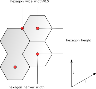
Hexagons are only slightly trickier to work with than squares. Computing face centers is simple. In Figure 11, there’s an i vector and a j vector. Going from hexagonal coordinates to world coordinates is a (very simple) matrix multiply:
⎛ x ⎞     ⎡ i.x j.x ⎤ ⎛ u ⎞
⎝ y ⎠  =  ⎣ i.y j.y ⎦ ⎝ v ⎠
Expanded out, that’s:
x = i.x * u + j.x * v
y = i.y * u + j.y * v
Figure 11 shows that for flat-topped hexagons, i is
(hexagon_narrow_width, 0.5*hexagon_height) and
j is (0, hexagon_height), so that give us
our values for i.x, i.y, j.x, j.y. (Pointy-topped hexagons will be silghty different.) The resulting code is:
# Face center
x = hexagon_narrow_width * u
y = hexagon_height * (u*0.5 + v)
Computing vertices is also fairly simple. In the rest of the
article I’ve labeled hexagon vertices either L or R. These two
vertices occur half a hexagon width left or right of the center
of the hexagon face (see Figure 9), so all we have to do is add
or subtract hexagon_wide_width * 0.5:
# If x,y are the face center, we can adjust to find a vertex
case side
  when :L
    x -= hexagon_wide_width * 0.5
  when :R
    x += hexagon_wide_width * 0.5
end
When working with hexagons, treat face centers as primary, and vertices as secondary.
Going from hexagonal coordinates (u, v) to world
coordinates (x, y) was a matrix multiply. To go
from world coordinates back to hexagons, you can solve the
equations for (u, v). I’ll skip the algebra;
here’s the result for flat-topped hexagons:
u = x / hexagon_narrow_width
v = y / hexagon_height - u * 0.5
That works if you start with (x, y) at a face
center. If you have arbitary (x, y) it’s a little
more work. The simplest (but not most efficient) way is to
consider the computed (u, v) plus all neighbors and
determine which one is closest to the given world coordinate.
This approach works for all three grid types. If you are using
this for mouse selection, this is plenty fast enough. It can be
optimized further by looking more closely at the polygons.
Triangles
Triangles are sheared and split squares. Triangle vertices only use the shearing step, which creates rhombuses. To convert triangle vertices from grid coordinates to world coordinates, multiply by the axis vectors i and j:
⎛ x ⎞     ⎡ i.x j.x ⎤ ⎛ u ⎞
⎝ y ⎠  =  ⎣ i.y j.y ⎦ ⎝ v ⎠
Expanded out, that’s
x = i.x * u + j.x * v
y = i.y * u + j.y * v
To convert triangle face coordinates to world coordinates
involves an adjustment. For face (u, v, L/R) first calculate the world coordinates of the lower left vertex, (u, v). Then for an L face, add (1/2 * i, 1/3 * j) to the lower left vertex location. For an R face, add (i, 2/3 * j) to the lower left vertex location. The result will be the center of the face.
To convert from world coordinates to triangle vertices, first find the lower left corner of the rhombus (u, v) using algebra, or by inverting the i.x,j.x,i.y,j.y matrix. The rhombus contains two triangle faces. To determine which face the point is in, look at the edge that divides the two triangles inside each rhombus (edge “E” in Figure 10). If frac(u) + frac(v) < 1.0, the point is on the left of the line, and is therefore in the L face; otherwise it is in the R face.
When working with triangles, treat vertices as primary, and face centers as secondary. This is the opposite of how we treat hexagons.
More#
Distance formulas on a square grid are well known (manhattan, euclidean, diagonal distance). Distance on a hex grid using this coordinate system uses an extension of the two-axis coordinates into a third axis, and I have the formula on my hex grid page[11]. Distance on a triangle grid is something I explore here[12]. This article from symbo1ics[13] has more math for triangle grids.
What else would you like to see me include in this document? Was anything confusing? Incomplete? Incorrect? Let me know.
The diagrams on this page were produced by implementing some
of the grid coordinate algorithms in Ruby[14], then generating
SVG[15], then
converting SVG to PNG[16] using Inkscape[17]. For a few
diagrams, I manually added annotations from within Inkscape.
My Ruby code is here. You can get
any of the SVG diagrams by changing .png in the
URL to .svg. If you’d like to use my diagrams,
please email me.
There are some things I didn’t find a place for, but might be of interest. Mathematicians have found five types of grids in 2D space[18]: squares, triangles, hexagons[19], rectangles, and parallelograms. However only squares, triangles, and hexagons are regular polygons. Spiral Honeycomb Mosaic[20] is an interesting way to assign numbers to hexagons in a hexagonal grid. It results in bizarre properties.