I have tons of notes about the SimBlob project, but they were all on paper. I transferred them to the web [Aug 2002]. This page has notes for both SimBlob 1 and SimBlob 2, and it also has notes about what I actually implemented in SimBlob 1 and SimBlob 2. Some themes you may notice:
- I look for general algorithms that can be used for a variety of purposes.
- I look for algorithms that don’t directly produce the effect I want, but instead result in the effect emerging naturally from the rules. I hope these algorithms will lead to a less brittle, more adaptive simulation.
I also counted how many pages of notes I have written about each aspect of the game.
- 21 pages - about graphics / UI
- 23 pages - about the game world / simulation
- 2 pages - about user documentation
I spent much of my time (and more than half the code) on graphics / UI issues. At the time (1995), game graphics took more effort because the libraries were designed for applications and didn’t offer much in the way of sprites, textures, transparency, lighting. OpenGL and DirectX are really nice to have these days. In future games I’ll be able to spend more time on the important stuff.
- Download SimBlob 2 - OpenGL + GLUT, 3D hardware recommended. It should compile in both Linux and Windows/Cygwin.
- Screenshot 1
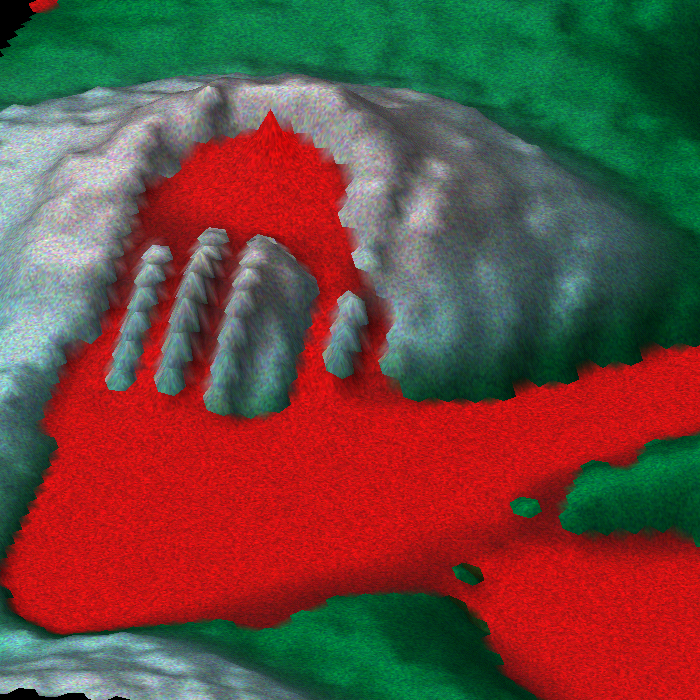
- Screenshot 2 (volcano)
- Screenshot 3 (lake)
- Screenshot 4 (rivers)
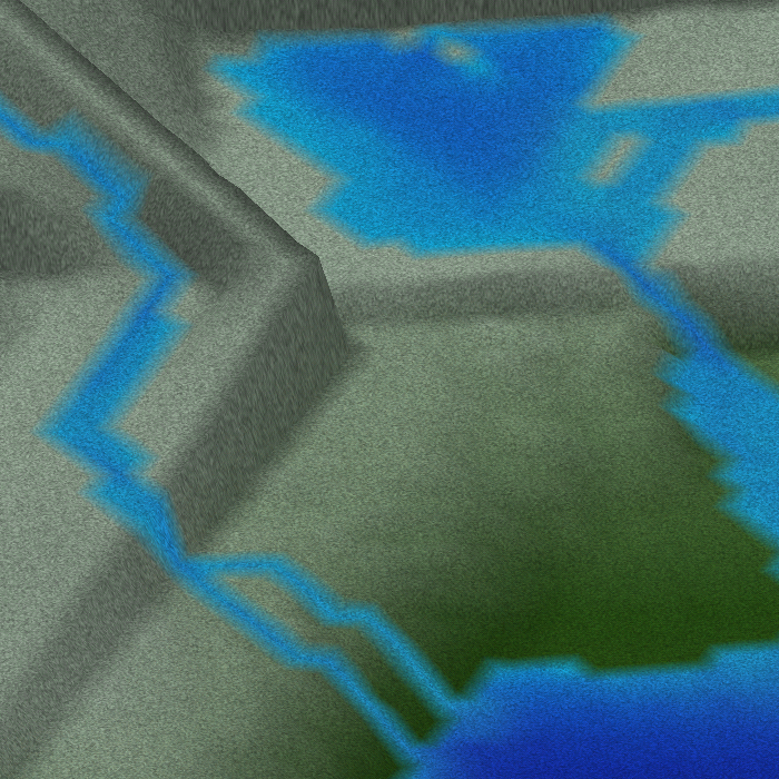
- Screenshot 5 (variable width river)
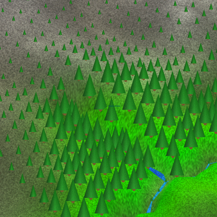
- Screenshot 6 (forest)
SimBlob 2 - Rendering
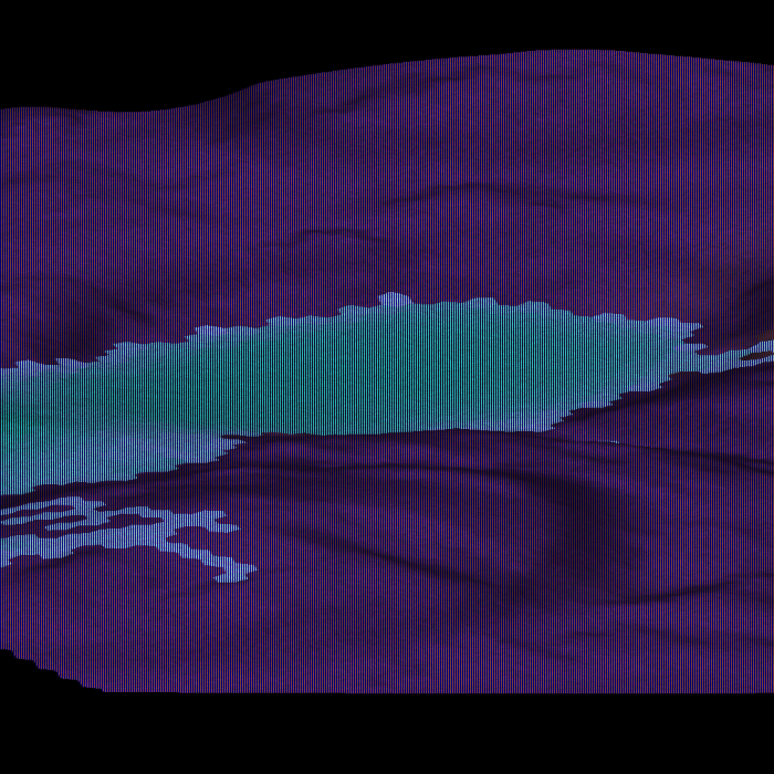
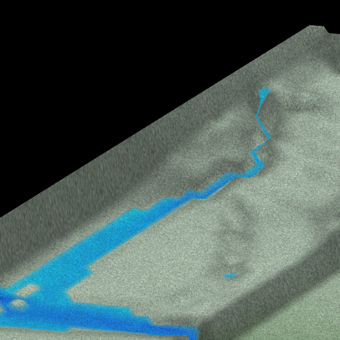
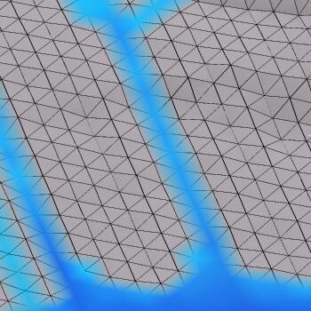
In the first version of SimBlob 2, each hexagon was drawn as six triangles. Each triangle consists of the center of the hexagon and two vertices. For each vertex, the z coordinate is the average of the z coordinates of the three hexagons that share the vertex. (If you think of the triangle formed by the centers of those three hexagons, then you can see why averaging the z coordinate works.) Unfortunately you can get rendering artifacts by taking this approach.
The image to the right illustrates several artifacts of rendering hexagons as six triangles. Look closely at the mountains to the left of the canyon. Each hexagon forms its own peak. You can’t build a straight ridge this way. Similarly, you can’t build a straight canyon; instead, the bottom of the canyon is bumpy. Let’s say the canyon has z=0 and the surroundng land has z=1. The vertices of the hexagons of the canyon will alternate between averaging 1 canyon hex and 2 ridge hexes (resulting in z=2/3) and averaging 2 canyon hexes and 1 ridge hex (resulting in z=1/3).
The zig zag effect isn’t only a problem for drawing terrain; rivers don’t look right either. The river in the canyon shows an awful rendering artifact: the water is creeping up the canyon walls. The river outside the canyon also shows a rendering artifact: it alternates between narrow and wide.
Another problem with the first rendering engine is that you can see land underneath water. In the above image, you can see a little bit of the canyon that the water is in. This is because the ridge hexes are partially drawn going down into the canyon. However, the ridge hexes have no water on them. So you end up rendering part of the canyon with no water on top.
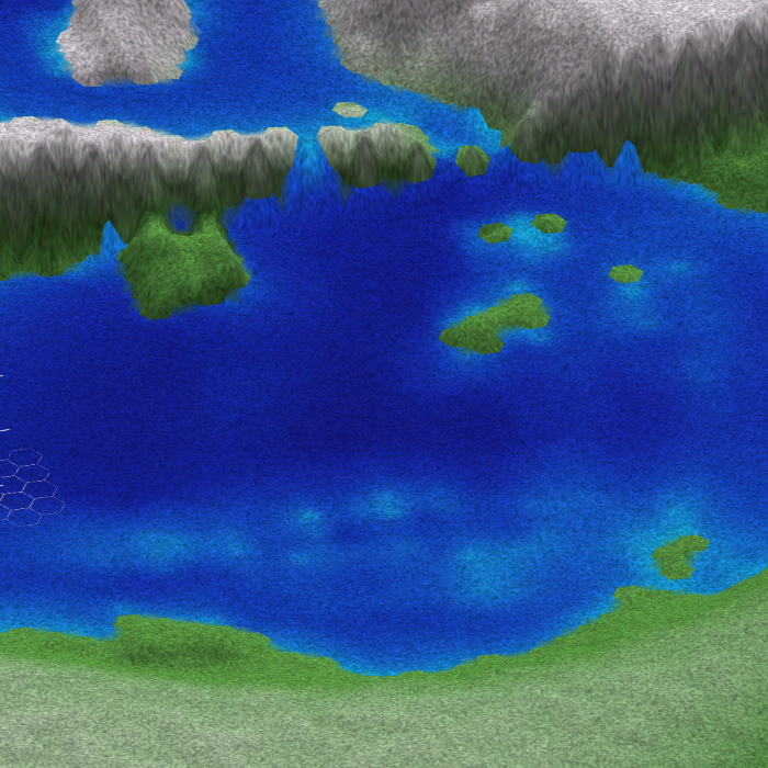
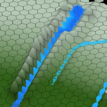
My second rendering engine draws triangles between the hexagon centers. The simulation objects are on the lines instead of in them. In the image to the right you can see the river follows the lines; in the first rendering engine, the river went between the lines. There is some connection here to Western games (Chess, Checkers) that put pieces in the squares and Eastern games (Go, Chinese Checkers) that put pieces on the lines. SimBlob’s simulation still occurs within hexagons, but the rendering of terrain and water is based on triangles between hexes. Making this work well is tricky. However, I found it to be worth it — not only do I get rid of many rendering artifacts, I also get approximately 30% faster rendering. I will still need to draw hexagons occasionally. To make these hexagons work properly, they need to be rendered as twelve triangles instead of six. Each triangle will be formed by the hexagon’s center, a vertex, and the midpoint of an edge.
The duality between hexagonal grids and triangular grids is quite interesting. In SimBlob, I take the centers of the simulation hexagons to get the vertices of rendering triangles. You can also take the centers of the rendering triangles to get the vertices of original simulation hexagons. My friend John Lamping suggested taking the midpoints of the edges of the rendering triangles to subdivide each triangle into four smaller ones. If you then take the centers of those smaller triangles, you form a small hexagonal grid -- one that’s rotated relative to the original grid! I ended up not using the subdivision because it made worse the problem of seeing land under water.
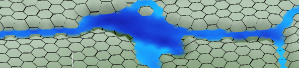
Rendering with triangles also helps with the problem with seeing land underneath water because we are drawing water all the way to the next hexagon. The problem of water “climbing” up the side of a hill is easier to solve when rendering with triangles, but it’s not automatic. The key is, for every hexagon that does not have water, lower its z coordinate (for water rendering only) to the lowest z coordinate of its neighbors. Screenshot 5 above shows the result.
Read more: vterrain[1].
SimBlob 1 - Geography#
First level: mountains, valleys, rivers, lakes, etc.
Second level: minerals, forests, farmland, etc.
Third level: water flow, erosion, flooding, etc.
Unorganized links:
- water flow over terrain, hex grids[2]
- water flow[3]
- introduction to fluid simulation techniques[4]
- more water flow[5]
- erosion[6], flooding, etc.
- Sediment capacity is water velocity to the third or fourth power; I didn’t model this at all in SimBlob 1, and used square of velocity in SimBlob 2.
- fluid motion[7]
- Boussinesq approximation[8] for water wave simulation
- oxbow lakes[9]
- types of erosion[10]
- erosion simulation[11]
- erosion in Tribal Trouble[12] {link broken but they released their game open source https://github.com/sunenielsen/tribaltrouble so maybe it’s somewhere there?}
- water flow (PDF)[13] article, a 3D water flow (PDF)[14] article
- deciding on vegetation/snow/etc. based on terrain characteristics[15]
- stable fluid simulation applet[16] (and original paper[17])
- Stable, Circulation-Preserving, Simplicial Fluids[18] (may not be practical for real-time simulation)
- Meandering Stream model the result of dam construction[19]
- Jos Stam’s paper[20] and source code[21] and notes on Stam’s method[22]
- particle-based fluid simulation[23]
- GPU-based water simulation[24]
- research into vegetation and rivers[25]
- WebGL water flow and erosion demo[26]
- water erosion on a heightmap[27]
- redditor who’s doing something similar[28]
- Soil physics[29] (fluid dynamics, groundwater, soil heat, aquifers)
At first, my plan was to have these tile types: Construction Yard, Road, Bridge, Farm, Homes, Business, Industry, Mine Forest, Water, Grassland, Desert, Hills, Mountains, Spring, Tower, Barracks, TankFactory, PowerLine, PowerPlant, Wall, Gate, BusStation, TrainStation. Construction Yard would require materials to build new objects. Those materials come from Industry, which gets raw materials from Forest and Mine.
As I started going into details I realized I need combinations of these, like a flooded farm on hills. Also, to make good water flow I needed to handle more than 4 elevations. So I switched to using 256 elevations (instead of Grassland/Hills/Mountains) and abandoned Desert. I put 256 levels of water (including 0) on every tile. I also remembered that I need to start simple, so I started with just Road on the first layer, Water on the second layer, and Altitude on the third layer. That simple set of tile data took a lot of implementation time. I’m glad I abandoned most of the tile types and just focused on the basics.
SimBlob 1 - Weather
Weather is a major influence on the environment. BlobCity has no weather simulation. The rivers come from randomly placed springs. The grass and trees are equally distributed at any particular altitude. I wanted to simulate some aspects of it in order to create these sorts of effects:
- The types of vegetation depends on rain and temperature. (Desert, grass, swamp)
- Rain feeds underground reservoirs, which can be tapped by wells.
- Forested areas absorb more water, leading to fewer chances of floods.
-
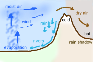 Mountain ranges cause “rain shadows”. As air rises, it
cools. Cold air can’t hold as much moisture as warm air.
Moist, warm air rising up a mountainside will cool and dump
some of its moisture as rain. On the other side of the
mountain, the dry air warms up more easily (it’s easier to
heat air than water), causing the air to be hotter than it
originally was.
Mountain ranges cause “rain shadows”. As air rises, it
cools. Cold air can’t hold as much moisture as warm air.
Moist, warm air rising up a mountainside will cool and dump
some of its moisture as rain. On the other side of the
mountain, the dry air warms up more easily (it’s easier to
heat air than water), causing the air to be hotter than it
originally was.
- Snow stores water during the winter and releases it in the spring. The rate of release depends on temperature, so temperature variation can lead to floods. See this page[30] for some details.
- Both rain and snowmelt feed rivers. The number and size of rivers should depend on the sources of water. River sizes may vary throughout the year.
To get some of these effects, I could need to keep track of data at every map location:
- Surface water
- Underground water (and maybe its depth)
- Snow level
- Humidity of air
- Temperature (maybe ground + air)
- Wind velocity (speed + direction)
The simulation rules would be:
- Absorption. Surface water turns into underground water. Depends on amount of surface water, type of surface (roads are less permeable than soil), amount of underground water.
- Seepage. Underground water turns into surface water. (Springs) Depends on amount of surface water, type of surface, amount of underground water. Seepage is rare. We probably need to have a surface opening for this to work. Also, in real life it depends on water pressure, which we aren’t simulating, so we’ll have to fake it.
- Evaporation. Surface water turns into humidity. Depends on temperature, humidity, vegetation. (Higher temperature, lower humidity, more vegetation leads to more evaporation.) Does not depend on amount of surface water (volume); depends on the surface area, which is roughly constant for a map location. Evaporation reduces surface temperatures. Also see this[31].
- Rain/Snow. Humidity turns into surface water. Depends on temperature, humidity, and whether it’s raining. (Lower temperature, higher humidity leads to more rain.) Once rain starts, it persists. That’s how we avoid perpetual drizzle in the equilibrium between evaporation and rain. If the temperature is low enough, we will have snow instead of rain. (What about ice? I decided not to worry about it.) Rain also decreases temperatures (which may be a factor in making rain persistent, since lower temperatures lead to more rain).
- Wind. Wind moves humidity and temperature from one map location to another.
- Plant Growth. Plants take underground water and use it to grow.
- Plant Death. Parts of plants constantly die (often by being eaten). The rate depends partially on temperature. High temperatures cause plants to wither. Very low temperatures cause plants to freeze (maybe depending on underground water; investigate hard freezes).
One possible extension is to treat underground water just like surface water in its ability to flow. To do this, we’d want to keep two altitude levels: one is the base altitude (the level of bedrock); the other is the surface altitude (the level of the soil). In real life there can be many layers of different types (clay, rock, etc.) but impermeable rock + permeable soil is the simplest way I can think of to get some underground water flow. With this you could have underground reservoirs. Seepage would occur whenever underground water level exceeds the depth of the soil.
SimBlob 1 - Economy
BlobCity
The BlobCity model was fairly simple. Farms consume labor and produce food. Houses consume food and produce labor. Labor and food are transported on roads to markets. Labor is taxed. With that money the player builds more objects.
The Silver Kingdoms: Objects
Each object can take some (discrete) set of inputs and produce some (discrete) set of outputs.
- Farm: 1 Water -> Corn
- Farm: 1 Water -> Barley
- Farm: 1 Water -> Wheat
- Farm: 2 Water -> Animal Feed
- Farm: 3 Water -> Fruits/Vegetables
- Iron Ore Mines: 0 -> Iron Ore
- Coal Mines: 0 -> Coal
- Silver Mines: 0 -> Silver
- Quarry: 0 -> Stone
- Logging Camp: (forest) -> Log
- Windmill: (wind) -> Power
- Waterwheel: (water) -> Power
- Builders: 1 Stone -> Road
- Builders: 1 Stone -> Wall
- Lumber Mill: 1 Log + 1 Power -> Wood
- Cottom Farm: 0 -> Cotton
- Flour Mill: 1 Corn + 1 Power -> Flour
- Bakery: 1 Flour -> Bread
- Tavern: 1 Fruit/Vegetable + 1 Water + 1 Meat -> Prepared Meal
- Cattle/Pig/Chicken Ranch: 1 Animal Feed -> Meat
- Sheep Ranch: 1 Animal Feed -> Wool
- Forge: 1 Iron Ore + 1 Coal -> Iron
- Blacksmith: 1 Iron + 1 Water -> Tools
- Armoury: 1 Iron + 1 Wood + 1 Water -> Armor
- Armoury: 1 Iron + 1 Wood + 1 Water -> Weapons
- Textile Factory: 1 Wool + 1 Power -> Clothing
- Textile Factory: 1 Cotton + 1 Power -> Clothing
- City: Bread -> 0
- City: Clothing -> 0
- City: Tool -> 0
- City: Wood -> 0
Labor is used everywhere.
The Silver Kingdoms: Production Model
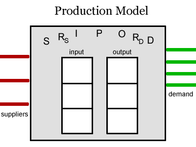
Each game object will fit into the production model shown on the right. There are some number of links to suppliers (S), which are other objects. There are some number of links to demanders (D), which are also other objects. The D links from one object link to the S links of the next object. There are reliability functions for the supply and the demand (RS, RD) that take the raw supply and express how quickly the product decays. (For example, fruit would decay quickly, and stone would never decay.) The input inventory I and the output inventory O act as buffers. The production function P expresses how to take transform inputs nito outputs (and how long it takes).
Every game tick, if there isn’t enough input inventory, the object has to buy some from suppliers. The choice of where to buy depends on the cost of acquiring the goods (the supplier’s charge plus the transportation cost). As goods are bought, the supplier may increase the charges, so we have to re-evaluate the cost after each item.
Every game tick, if there is demand and output inventory, try
to sell some. By remembering the average demand price, we can
consider keeping some of the goods in inventory (but discount
future income by RD and also by some
“inflation” factor).
Thoughts from others
Jeremiah McCall (author of this book[32]) gave me some good historical notes: In early societies, cities consume resources from the surrounding areas, and don’t produce much. Also, it took a lot of farmers to support one city dweller, so most people had to be farmers. Irrigation canals improved farm yields. As more food was produced per person, more people could move to cities. As cities grew, they could start producing their own goods. Transportation also affected the balance. Poor transportation limited city size because cities could not import food from farther away. Transportation on water routes was an important (and often faster) alternative to land routes.
Will Wright (of Maxis) said that in SimCity cities, industrial and commercial zones change importance as the city grows. Commerce is proportional to the city size (it’s probably superlinear). Industry is sublinear. So when the city is small, industry matters a lot; when it’s large, commerce matters a lot. SimCity 4 uses regional economies[33] to make the simulation richer. {link broken, thanks EA! :-( }
City Placement
Where do cities form? They evolve in places with good farmland, good water, good access to roads, good access to minerals, etc. But then they evolve, sometimes in ways not consistent with their original reason for placement. I’d like to experiment with roads and cities co-evolving. As cities grow, they build roads to important nearby places (other cities, natural resources, etc.). As roads grow, city growth starts to follow the roads. Roads are influenced by the landscape (slope, land type, etc.).
Read more: Central Place Theory[34] attempts to explain placement of cities, businesses, etc. Interestingly, on a flat piece of uninteresting land, placement follows a hexagonal pattern[35], Co-evolution of density and topology in a simple model of city formation [PDF][36].
Geography and Economics
In basic high school economics, we don’t get to learn about the effect of geography on economics. It is assumed that all the businesses compete on an equal ground—that there’s no cost of transporting goods around. The analysis never covered what happens when all the workers live in Paris and all the businesses are in London. The equations would come out looking like everything was just fine. But when businesses and workers are located in different places, it makes quite a difference in economic decision making.
The first thing to consider is that businesses can assign a value to being in each location. (In economic speak, this is called “rent”, but because common people use that term differently, I’ll call it “location value”.) For example, a large bank may find it very valuable to be in the city center and not very valuable to be in a rural area. In contrast, a farm may find it valuable to be in a location with good soil and access to irrigation channels. For each location, the best business to move in is the one with the highest location value. For each business, the best location to move into is the one with the highest location value minus the cost of being there (what we commonly refer to as ... rent). Although the business is the one making the decision, the locations can set their rent, so they can exert an influence over the choice made by the businesses. A location wants to set the rent high enough to make money (and exclude low-value businesses) but low enough to attract the business to that location instead of other locations. This requires complicated analysis, right?
“A good analogy is the scattering of certain types of seeds by the wind. These seeds may be carried for miles before finally coming to rest and nothing makes them select spots particularly favorable for germination. Some fall in good places and get a quick and vigorous start; others fall in sterile or overcrowded spots and die. Because of the survival of those which happen to be well located, the resulting distribution of such plants from generation to generation follows closely the distribution of favorable growing conditions. So in the location of economic activities it is not strictly necessary to have both competition and wise business planning in order to have a somewhat rational location pattern emerge; either alone will work in that direction.” (Edgar M. Hoover, The Location of Economic Activity 1948, page 10)
In a simulation game, we can use experimentation instead of analysis. Each location can set a rent that’s fairly high, then lower it if it can’t get any business to move in. Each potential business can pick some small set of locations, try to estimate how profitable it would be in that location, and pick the best one. The potential business can also have an idea of how profitable it expects to be, and if none of the locations are profitable enough, it can wait. (The expected profit can be a moving average of the better locations evaluated by similar potential businesses in that area.)
The idea of experimentation works after the business has been placed, too. Businesses have to select suppliers and prices. They can try varying these and see if things improve. If they do, they keep the new values. If not, they go back to the old values. This can be combined with reinforcement learning[37] if desired.
As AI agents experiment with their businesses, personality comes into play. Given variability in profit levels (“location X may produce a profit from Y to Z”), an agent may be:
- Cautious. Maximize the low end of the profit estimate.
- Reckless. Maximize the high end of the profit estimate.
- Rational. Maximize the expected profit.
- Regretful. Minimize the difference between the high end of the profit estimate and the expected profit.
The second big issue to consider in combining geography and economics is transportation cost. Heavy goods cost more in general to transport than light goods. Longer distances generally cost more to traverse. However, the transportation costs are not directly proportional to distance and weight. Transportation along rail lines means that locations near the train stations are better than locations far from the stations. Transportation along roads means that locations near roads (even better, highways) are better than locations far from them.
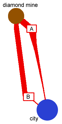
Consider for example the diamond industry. Hundreds of tons of rock are mined to find a few grams of diamonds[38]. The cost of transporting the rock (thick red line) is much higher than the cost of transporting the diamonds (thin red line). To minimize costs, we want to place the processing plant near the diamonds. The problem with this simplistic model is that it leads to uninteresting games, because the optimal decision for each business is to either be as close to the city as possible or as close to the source of materials as possible. When the transportation cost ratio between the input and the output is high, the business prefers being near the input. When the ratio is low, the business prefers being near the output.
We can annotate the cost model with the cost of transporting workers. Although the business may not pay this cost directly, it has to increase salaries to convince workers to travel far from home. (This is why people working on off-shore oil rigs get paid more.) Even more interesting, labor costs don’t rise linearly (more below). This means that the optimal location for a business is often but not always at one end or the other, which makes for a more interesting game.
Why don’t labor costs increase linearly, like transportation costs for goods? With labor you are buying a person’s time. Time is limited. When you have 24 hours in a day, and 8 are sleeping, 2 are eating, and 8 are working, you have plenty of free time for travelling to work and leisure activities. A faraway business essentially has to buy leisure or other types of time from the worker and convert it into travelling time. When there are 6 hours of leisure time, this is easy (for most workers). When there’s only 1 hour of leisure time left, it’s much harder (more expensive) to convince the worker to give that up. So the cost to the business is fairly low for a while, but rapidly increases as the worker gets closer and closer to having 0 free time. In the diagram on the right, you can see the line between the city and A is narrow for a while and rapidly increases far from the city.
A simple model for leisure time involves making the change in
salary inversely proportional to the loss of free time.
Assuming total time k is fixed, we can say that
commute time c plus free time f
equals k. The change in salary is proportional
to 1 ÷ f, or 1 ÷
(k-c). The total salary is the integral of this, and
comes out to Log[k] - Log[k-c]. As
c approaches k, the
-Log[k-c] term approaches infinity. (This isn’t
quite right, because the worker might be willing to give up
sleep or other parts of the day.) In this simple model, you
can’t ever buy the worker’s last free minute.
We replace the simple transporation cost ratio model with a model involving forces pulling the business toward the various forms of input (raw materials, labor). The ideal location will be influenced by all the inputs. What is the cost of buying a worker’s leisure time? It’s harder to eat up leisure time when there are lots of other, nearby jobs available. So the ideal business location will change as unemployment levels change. The forces also change unevenly when transportation costs (new technology, new roads, new rail lines) change. The business that was ideally located several decades ago may no longer be ideally located. This opens up opportunities for new businesses. All of this is good potential for a rich simulation game.
Read more: Rent and Gradients[39] and Transportation theory algorithms[40] and StarPeace economic modeling[41].
SimBlob 1 - Military
Model
Since military is not a large part of BlobCity, I decided to make things relatively simple. Soldiers are recruited from the civilian population. Instead of controlling individual soldiers, you control squads of them. The squads are built automatically as you recruit more soldiers. (If there are squads that aren’t full, the recruits will fill them; otherwise, new squads are created.) Soldiers are alive or dead---no wounded soldiers, healing, etc. You can get the same effects as wounded soldiers at the squad level---after a battle, the squad isn’t full. To heal them, you take them back to base, where new recruits fill the squad. Each soldier has a skill level which increases over time.
Troop Formations
In a game about alien blobs on Mars, you can make new rules for culture and society that don’t match what you see on Earth. In particular, you can shape the society in a way that makes it easier to simulate and more fun to play. Troop formation has a long history on Earth. Instead of simulating that, I wanted to first find cool algorithms, then see if they would produce “interesting” movement patterns.
Flocking is one alternative to standard troop formations. Each soldier watches the behavior of nearby soldiers and uses simple rules to determine how to move. Although no one is actively creating a formation, the soldiers end up creating a formation anyway. Flocking patterns are observed in birds and fish (not human soldiers) on Earth, but why not in blobs on Mars?
Another source of inspiration is molecular forces. Atoms at
least a certain distance apart are attracted to one another.
When they get closer than that distance, they repel. (The
formulas for this involve an attractive force proportional to
d^-6 and a repulsive force proportional to
d^-12. For small d, the repulsive
force dominates.) Soldiers near each other would form
“molecular” bonds between them and they would stay together
unless pulled apart by an equally strong force. They would
also maintain their distance.
Orders
When I started SimBlob, I played games that had manual troop orders. You could select a group of soldiers and tell them to move somewhere, to attack some object, etc. Since SimBlob isn’t mainly a military game, I wanted to automate some of that, so I planned (but never implemented) these orders:
- Attack. [some target]
- Defend. [some perimeter]
- Patrol. [two or more points]
- Explore. [starting point]
- Move. [destination point]
- Retreat. [gathering point]
These days, games do offer these sorts of commands, and after playing them, I’ve decided that I really like the idea and want to implement it in my next game. I also want the squads to act on their own if you don’t want to give them orders.
Influence Maps
Each map location can keep a “scent” that records which team has last been there. The scent fades over time, and scents spread out into neighboring map locations. Soldier pathfinding can use the scents to either avoid or head towards enemy units.
Scenarios
The original goal for SimBlob was ambitious: as you built your city, you’d eventually run out of space and you’d use your military to comquer land from adjacent cities. (The walls were a big part of that.) However, as SimBlob evolved into BlobCity, I dropped the idea of city states (mainly because I knew I wouldn’t have time to develop a good AI). BlobCity is an open-ended game with the player alternating building and dealing with environmental disasters (both natural ones like floods, volcanos, fires, and man-made ones like overforestation, topsoil erosion). The military could be used to fight barbarian raids or organized enemies. This is one of the least fleshed out parts of the design, and it was never implemented.
SimBlob 1 - Game Alternatives
BlobCity uses each game tile for a farm, house, market, etc. An alternative would be to zoom out and put an entire town into a tile. One problem I found in BlobCity is that it’s hard to write code that looks at patterns. Humans can easily decide where a town is. Brains are very good at finding patterns. However, a computer algorithm has a much harder time. When a town is placed on a single tile, there’s a discrete object that can be used for the game simulation and AI. Discrete objects can have names and properties; fuzzy patterns are harder to deal with. Discrete objects also lend themselves to agent-based AI.
Discrete objects that I started thinking about: City (produces income, labor, and soldiers; consumes food), Mine (produces iron and coal; consumes labor), Farm (produces food; consumes labor), Lumber Yard (produces timber; consumes labor and nearby trees).
See this page for an overview of the SimBlob game ideas. The Silver Kingdoms was the most interesting to me. I haven’t really decided on many design aspects. Some of these can be considered to be different scenarios.
Player starts:
- Player starts with only money.
- Player starts with some objects (farms, industries, etc.).
World starts:
- World starts with nothing. The player has the opportunity to build it all.
- World starts with markets that sell some (or all) goods at high prices. The player has the opportunity to build businesses that sell lower cost or higher profit goods.
- World starts with industries. The player transports raw materials and goods to markets.
- World starts with cities. The player provides goods to the cities.
- World starts with base resources (farms, mines, lumber yards). The player takes those resources and produces goods.
Player actions:
- The player builds objects and roads.
- The player manages object growth.
- The player manages object connections (what farms does this market buy from?).
- The player buys land, improves it (walls, canals, gates, houses, commercial buildings), rents it out, or sells it.
- The player builds transportation routes (road, rail, ship).
- The player attacks other cities and industries to build wealth and power.
- The player sabotages other cities and industries by environmental disasters (floods, volcanos, fires)
Player building options:
- The player can build anything.
- The player can build industries that supply cities.
- The player can build cities only.
- The player can build markets and transportation systems.
There are a lot of interesting simulation questions to solve:
- Where do cities form? How do they grow?
- What goods do city inhabitants need?
- What role do small businesses (too small to be explicitly simulated) play?
- How are land values determined? Land is valued differently by different people. For example, a skyscraper owner values land near the city center a whole lot more than land out near the edge of the city. But a farmer values land based on its soil quality, access to markets, etc.
Miscellaneous Algorithms
Most algorithms work focuses on taking some input, solving the problem, and producing output. These are called offline algorithms. In contrast, online algorithms take the input a bit at a time and produce output a bit at a time. These are often more relevant to games programming. Another property that’s quite useful is incremental update. If the input changes a small amount, can we find the new answer with a small amount of work, or do we have to do all the work again? (The only version of this that’s covered by introductory algorithms books is sorting mostly-sorted input.) For most of the economic and geographic simulation in SimBlob, incremental update is very important. I also would like to find approximation algorithms. I usually don’t need to know exactly how much water flowed down the river. An approximation is just fine.
SimBlob 1 - Pathfinding
I spent a lot of time trying to figure out good pathfinding. In 1995, there wasn’t a lot of information on this topic on the web. I wrote up quite a few pathfinding notes[42].
City Growth
There is some research on city growth models. The basic data in the model is for each map location: land price, cost of building (depends on the terrain, mainly slope). I took notes on the basic growth rules they used:
- Spontaneous Growth. If the space is empty, a neighboring space is occupied, and the cost of building is low, occupy the space. Probability of using this rule is constant.
- Diffusive Growth. If the space is empty, a nearby (not necessarily neighboring) space is occupied, and the cost of building is low, occupy the space. This rule is pretty similar to Spontaneous Growth, but the probability of using this rule is proportional to the total population.
- Organic Growth. If the space is empty, several neighboring spaces are occupied, and the cost is low or medium, occupy the space. Probability is proportional to the total population. This rule is similar to Diffusive Growth but it allows higher population density to override the preference for low building costs. I think the two rules could be blended together into one.
- Road Influenced Growth. Pick a random occupied area. Find a nearby road. Travel some distance along that road. If the areas near that road are empty, occupy one of them. This rule allows new cities to form.
I may have some of the details wrong; if you catch an error please let me know! There are lots of these urban growth models being used to predict population growth of real cities. For more details, try this Google search[43].
SimBlob 1 - Road Building
In real life, most American cities have ended up using rectangular grid patterns. On the hexagonal map used in BlobCity, city grid road patterns don’t look right. I considered imposing some order on the road system[44] but then I decided on a subtler approach: I would let roads grow organically but give them influencing forces. On a hexagonal grid, that meant rewarding road hexes with two or three road connections and penalizing road hexes with four or more road connections. Zero or one road connections is a sign of a developing road; I didn’t want to reward or penalize it. I also inhibited road forces on non-road hexes if they had two adjacent neighbors with a road already on them (*). Non-adjacent neighbors with roads increased the chance of making the hex into a road. (The rules for non-road hexes are weird; you might want to draw it out to see why it helps.) The result is a pleasant looking system of roads[45].
I also put in some rules to influence the spacing of roads. Roads that are spaced too close together aren’t utilizing the land well; roads that are too far apart don’t provide enough access to the houses, markets, and farms nearby.
(*) It would be nice to take into account the age of the road here. If the road is old and only has zero or one connections, it may be a bad sign. There’s probably an alternate approach to this involving economics: newly built roads get some sort of “benefit credit”, the credit is used up over time, and they get “rewarded” for traffic. Roads with zero or one connector won’t get much traffic, so they will run out of credit and get removed.
Read more: Procedural Modeling of Cities[46] (PDF)
SimBlob 1 - Scheduling Work
In addition to the “sims” in the game (which were invisible and not individually tracked), there were “blobs” that were simulated individually. Worker blobs could build objects (both those requested by the player and those requested by the sims), cut down trees, and put out fires. So the problem is that there’s a set of tasks (locations where the player wants to build something, or fires to be put out) and we want to schedule the blobs to work on each task. First come first serve didn’t always work well---the player would create one set of objects in one place then another set in another place. If there were two blobs, one close to the first project and one close to the second, they’d both go to the first project, finish it, then both go to the second. A more efficient approach would be for the blobs to go work on what’s closest to them. However, that doesn’t always work either---if the blobs are near each other, they’ll all end up working on the same project, and travel to the next project together, which keeps them together. Once they get together, they’ll never split up and work on separate projects. When there’s small amounts of work being generated all the time all over the map (this happens when the city is large and residents everywhere want to build new things), the blobs spent almost all their time travelling.
The approach I used in BlobCity was to divide the world up into 8x8 sectors. (I also considered dividing the world up into hexagonally shaped sectors, but it was more work and didn’t seem to be much better.) Each blob would decide which sector to work in. The desirability of working that sector depended on the amount of work in that sector (more is better), the number of blobs already wanting to work there (more is worse), and the distance from the blob’s current location to that sector (higher is worse). This algorithm worked reasonably well.
This problem turns out to be similar to the k-server problem[47], except that we have a little bit more flexibility in that we don’t require that a blob immediately service a request.
Response Curves
Many times I’ll want a non-linear response to something in the simulation. Crop yield depends on water, soil, fertilizer, etc., but increasing just one of these won’t increase crop yield much. The right balance matters. Functions that I use to give me various types of responses are:
-
Rate of Change.
You often see people say “30% more XYZ!” Percentages are a decent way to describe small changes. However, there are four commonly used ways to express the change from
xtoy: percent increase ((x-y)/y), ratio increase (x/y), percent decrease ((x-y)/x), ratio decrease (y/x). All of these have the problem that ifxoryis 0, you are in trouble!So what I use instead is
y/(x+y). When it’s 0.5, there’s no change; 0.0-0.5 means a decrease; 0.5-1.0 means an increase. No dividing by zero. -
Exponential Decay.
A cheap way of keeping a running average.
xavg := (1-a)*xavg +
            a*xmeasurement
. The parameteracontrols how quickly new measurements are factored into the average. This is one of the components of Proportional + Integral + Derivative control systems[48]. -
Logarithmic Growth.
There are many things in life that having 2x of isn’t twice as good as having x of. Time, money, food, tv channels are examples. One way to model these “diminishing returns” in a game is
benefit := log(quantity). -
Diminishing Returns. (alternative)
y := b * a / (a + x). The base level isb, but asxincreases,ydecreases. The parameterais a way to tune how quicklyydecreases—whenx = a, the outputywill be half of the base value. Yes, this formula involves a divide, but it’s cheaper than a logarithm. -
S-curve.
An S-curve gives low rates of return at low values of
x, good returns at medium values, and low returns at high values. You can build a polynomial version over0 <= x <= 1by settingf(x) = a * x3 + b * x2 + c * x + d, then solving for these constraints:f(0) = 0,f(1) = 1,f'(0) = 0,f'(1) = 0, wheref'(x)is the first derivative off(x). When you do that, you’ll get the coefficients needed for your polynomal.f(x) = -2 * x3 + 3 * x2.This technique of building polynomials from constraints is quite useful.Another way of getting an S-curve is to use a sigmoid function[49]. The advantage of the sigmoid is that it works for all
x, not only0 <= x <= 1, and never quite reaches minimum or maximum. However, it includes both a divide and an exponential. -
Gaussian Distribution.
See this page[50]. The integral of the Gaussian is also interesting—it’s another kind of S-curve! (But it’s icky to calculate.)
-
Lotka-Volterra Equations.
These are used for simulating competing populations. Population X increases exponentially (birth rate is greater than natural death rate):
x := (1 + a) * x(whereais a small number like 0.1 or 0.01). Population Y feeds on population X, and therefore birth rate depends onx:y := y + d * x * y. The X’s are dying as the Y’s feed on them:x := x - b * x * y. Population Y also has a death rate that does not depend on population X:y := (1 - c) * y. See graphs here.[51]
In general, I try to use responses that are sublinear. As you put more and more resources into something, you get diminishing returns. This negative feedback leads to stable situations. On the other hand, I don’t always want to reach an equilibrium, and things like the Lotka-Volterra equations can help there.
SimBlob 2 - Reaction-Diffusion Patterns
In chemistry, there are unusual patterns that can be generated from simply mixing two chemicals together. Starting with a random mixture of chemicals, the reaction rules naturally generate patterns. The rules are fairly simple:
- Reaction. Chemical A breaks down chemical B if the concentration of B is high. Chemical B is produced if the concentration of A is high.
- Diffusion. Both chemicals flow from high concentration to low concentration.
Depending on how fast the two chemicals react, you can get many different patterns (like stripes and spots in animals). See plate 2 on this page[52] to see some of the patterns. Explore more of that site to see lots of other patterns that can be generated by simple rules.
I was hoping to use some of these ideas in city growth rules. There are probably some interesting ways to use reaction-diffusion to decide how residential and commercial areas are laid out.
SimBlob 1 - Traffic Simulation
There are many research and commercial systems that simulate traffic. There is a neat game called Mobility[53] that focuses on this topic. However, most of the models are too complicated for BlobCity, in which traffic plays a minor role. I couldn’t dedicate all the CPU power to just traffic. Instead, I used a water flow model. Houses produce “traffic” and push it out onto the closest road. Workplaces consume “traffic” and pull it from the closest road. Then I let the traffic “flow” from higher points to lower points. At some point I reach equilibrium. This tells me how much traffic there is on each segment of road. It’s not too realistic but it’s very simple and cheap to update.
Read more: SimCity uses trip generation[54] to figure out traffic. Also read SimCity 4 Automatons[55]. {links broken, thanks EA! :-( }
SimBlob 1 - Labor Simulation
Similar to traffic simulation, labor simulation in BlobCity is very simple. Houses produce “labor” and push it out onto the closest market. Workplaces (farms, lumber yards) consume “labor” and pull it from the closest market. The labor can flow along markets and roads from higher values to lower values. The amount of food produced at a farm depends on the labor value there. Houses with lower labor values (meaning the people there found jobs) are more likely to attract new residents.
New houses might be built where the labor pressure is too low (meaning there are lots of jobs). New workplaces might be built where the labor pressure is too high (meaning there are lots of workers). New roads might be built where the labor pressure is too high or too low.